Weighted Reductions

Xarray supports weighted reductions.

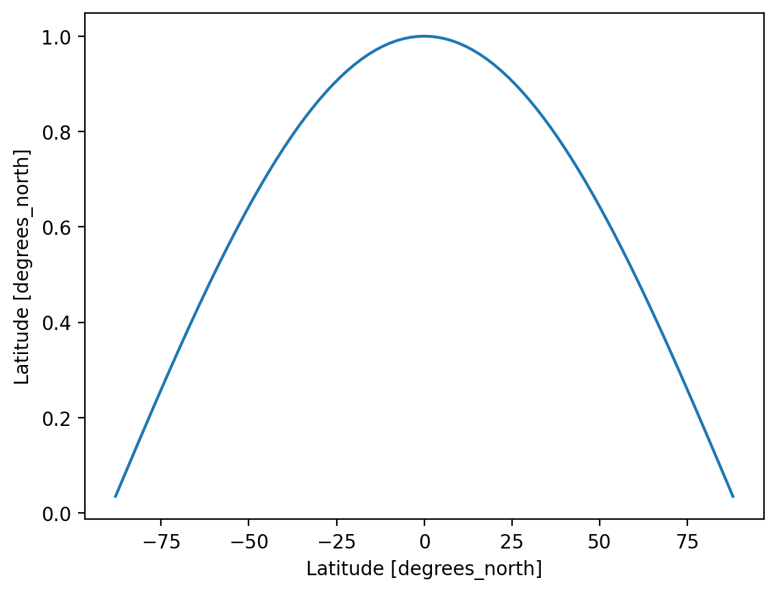
For demonstration, we will create a “weights” array proportional to cosine of latitude. Modulo a normalization, this is the correct area-weighting factor for data on a regular lat-lon grid.

import numpy as np
import xarray as xr
import matplotlib.pyplot as plt

%config InlineBackend.figure_format='retina'

ds = xr.tutorial.load_dataset("ersstv5")
ds

<xarray.Dataset>
Dimensions:    (lat: 89, lon: 180, time: 624, nbnds: 2)
Coordinates:
  * lat        (lat) float32 88.0 86.0 84.0 82.0 ... -82.0 -84.0 -86.0 -88.0
  * lon        (lon) float32 0.0 2.0 4.0 6.0 8.0 ... 352.0 354.0 356.0 358.0
  * time       (time) datetime64[ns] 1970-01-01 1970-02-01 ... 2021-12-01
Dimensions without coordinates: nbnds
Data variables:
    time_bnds  (time, nbnds) float64 9.969e+36 9.969e+36 ... 9.969e+36 9.969e+36
    sst        (time, lat, lon) float32 -1.8 -1.8 -1.8 -1.8 ... nan nan nan nan
Attributes: (12/37)
    climatology:               Climatology is based on 1971-2000 SST, Xue, Y....
    description:               In situ data: ICOADS2.5 before 2007 and NCEP i...
    keywords_vocabulary:       NASA Global Change Master Directory (GCMD) Sci...
    keywords:                  Earth Science > Oceans > Ocean Temperature > S...
    instrument:                Conventional thermometers
    source_comment:            SSTs were observed by conventional thermometer...
    ...                        ...
    creator_url_original:      https://www.ncei.noaa.gov
    license:                   No constraints on data access or use
    comment:                   SSTs were observed by conventional thermometer...
    summary:                   ERSST.v5 is developed based on v4 after revisi...
    dataset_title:             NOAA Extended Reconstructed SST V5
    data_modified:             2022-06-07

xarray.Dataset

• Dimensions:
  • lat: 89
  • lon: 180
  • time: 624
  • nbnds: 2
• Coordinates: (3)
  • lat
    (lat)
    float32
    88.0 86.0 84.0 ... -86.0 -88.0

    units :

    degrees_north

    long_name :

    Latitude

    actual_range :

    [ 88. -88.]

    standard_name :

    latitude

    axis :

    Y

    coordinate_defines :

    center

    array([ 88.,  86.,  84.,  82.,  80.,  78.,  76.,  74.,  72.,  70.,  68.,  66.,
            64.,  62.,  60.,  58.,  56.,  54.,  52.,  50.,  48.,  46.,  44.,  42.,
            40.,  38.,  36.,  34.,  32.,  30.,  28.,  26.,  24.,  22.,  20.,  18.,
            16.,  14.,  12.,  10.,   8.,   6.,   4.,   2.,   0.,  -2.,  -4.,  -6.,
            -8., -10., -12., -14., -16., -18., -20., -22., -24., -26., -28., -30.,
           -32., -34., -36., -38., -40., -42., -44., -46., -48., -50., -52., -54.,
           -56., -58., -60., -62., -64., -66., -68., -70., -72., -74., -76., -78.,
           -80., -82., -84., -86., -88.], dtype=float32)

  • lon
    (lon)
    float32
    0.0 2.0 4.0 ... 354.0 356.0 358.0

    units :

    degrees_east

    long_name :

    Longitude

    actual_range :

    [ 0. 358.]

    standard_name :

    longitude

    axis :

    X

    coordinate_defines :

    center

    array([  0.,   2.,   4.,   6.,   8.,  10.,  12.,  14.,  16.,  18.,  20.,  22.,
            24.,  26.,  28.,  30.,  32.,  34.,  36.,  38.,  40.,  42.,  44.,  46.,
            48.,  50.,  52.,  54.,  56.,  58.,  60.,  62.,  64.,  66.,  68.,  70.,
            72.,  74.,  76.,  78.,  80.,  82.,  84.,  86.,  88.,  90.,  92.,  94.,
            96.,  98., 100., 102., 104., 106., 108., 110., 112., 114., 116., 118.,
           120., 122., 124., 126., 128., 130., 132., 134., 136., 138., 140., 142.,
           144., 146., 148., 150., 152., 154., 156., 158., 160., 162., 164., 166.,
           168., 170., 172., 174., 176., 178., 180., 182., 184., 186., 188., 190.,
           192., 194., 196., 198., 200., 202., 204., 206., 208., 210., 212., 214.,
           216., 218., 220., 222., 224., 226., 228., 230., 232., 234., 236., 238.,
           240., 242., 244., 246., 248., 250., 252., 254., 256., 258., 260., 262.,
           264., 266., 268., 270., 272., 274., 276., 278., 280., 282., 284., 286.,
           288., 290., 292., 294., 296., 298., 300., 302., 304., 306., 308., 310.,
           312., 314., 316., 318., 320., 322., 324., 326., 328., 330., 332., 334.,
           336., 338., 340., 342., 344., 346., 348., 350., 352., 354., 356., 358.],
          dtype=float32)

  • time
    (time)
    datetime64[ns]
    1970-01-01 ... 2021-12-01

    long_name :

    Time

    delta_t :

    0000-01-00 00:00:00

    avg_period :

    0000-01-00 00:00:00

    prev_avg_period :

    0000-00-07 00:00:00

    standard_name :

    time

    axis :

    T

    actual_range :

    [19723. 81204.]

    array(['1970-01-01T00:00:00.000000000', '1970-02-01T00:00:00.000000000',
           '1970-03-01T00:00:00.000000000', ..., '2021-10-01T00:00:00.000000000',
           '2021-11-01T00:00:00.000000000', '2021-12-01T00:00:00.000000000'],
          dtype='datetime64[ns]')

• Data variables: (2)
  • time_bnds
    (time, nbnds)
    float64
    9.969e+36 9.969e+36 ... 9.969e+36

    long_name :

    Time Boundaries

    array([[9.96920997e+36, 9.96920997e+36],
           [9.96920997e+36, 9.96920997e+36],
           [9.96920997e+36, 9.96920997e+36],
           ...,
           [9.96920997e+36, 9.96920997e+36],
           [9.96920997e+36, 9.96920997e+36],
           [9.96920997e+36, 9.96920997e+36]])

  • sst
    (time, lat, lon)
    float32
    -1.8 -1.8 -1.8 -1.8 ... nan nan nan

    long_name :

    Monthly Means of Sea Surface Temperature

    units :

    degC

    var_desc :

    Sea Surface Temperature

    level_desc :

    Surface

    statistic :

    Mean

    dataset :

    NOAA Extended Reconstructed SST V5

    parent_stat :

    Individual Values

    actual_range :

    [-1.8 42.32636]

    valid_range :

    [-1.8 45. ]

    array([[[-1.8, -1.8, -1.8, ..., -1.8, -1.8, -1.8],
            [-1.8, -1.8, -1.8, ..., -1.8, -1.8, -1.8],
            [-1.8, -1.8, -1.8, ..., -1.8, -1.8, -1.8],
            ...,
            [ nan,  nan,  nan, ...,  nan,  nan,  nan],
            [ nan,  nan,  nan, ...,  nan,  nan,  nan],
            [ nan,  nan,  nan, ...,  nan,  nan,  nan]],
    
           [[-1.8, -1.8, -1.8, ..., -1.8, -1.8, -1.8],
            [-1.8, -1.8, -1.8, ..., -1.8, -1.8, -1.8],
            [-1.8, -1.8, -1.8, ..., -1.8, -1.8, -1.8],
            ...,
            [ nan,  nan,  nan, ...,  nan,  nan,  nan],
            [ nan,  nan,  nan, ...,  nan,  nan,  nan],
            [ nan,  nan,  nan, ...,  nan,  nan,  nan]],
    
           [[-1.8, -1.8, -1.8, ..., -1.8, -1.8, -1.8],
            [-1.8, -1.8, -1.8, ..., -1.8, -1.8, -1.8],
            [-1.8, -1.8, -1.8, ..., -1.8, -1.8, -1.8],
            ...,
    ...
            ...,
            [ nan,  nan,  nan, ...,  nan,  nan,  nan],
            [ nan,  nan,  nan, ...,  nan,  nan,  nan],
            [ nan,  nan,  nan, ...,  nan,  nan,  nan]],
    
           [[-1.8, -1.8, -1.8, ..., -1.8, -1.8, -1.8],
            [-1.8, -1.8, -1.8, ..., -1.8, -1.8, -1.8],
            [-1.8, -1.8, -1.8, ..., -1.8, -1.8, -1.8],
            ...,
            [ nan,  nan,  nan, ...,  nan,  nan,  nan],
            [ nan,  nan,  nan, ...,  nan,  nan,  nan],
            [ nan,  nan,  nan, ...,  nan,  nan,  nan]],
    
           [[-1.8, -1.8, -1.8, ..., -1.8, -1.8, -1.8],
            [-1.8, -1.8, -1.8, ..., -1.8, -1.8, -1.8],
            [-1.8, -1.8, -1.8, ..., -1.8, -1.8, -1.8],
            ...,
            [ nan,  nan,  nan, ...,  nan,  nan,  nan],
            [ nan,  nan,  nan, ...,  nan,  nan,  nan],
            [ nan,  nan,  nan, ...,  nan,  nan,  nan]]], dtype=float32)

• Indexes: (3)
  • lat
    PandasIndex

    PandasIndex(Index([ 88.0,  86.0,  84.0,  82.0,  80.0,  78.0,  76.0,  74.0,  72.0,  70.0,
            68.0,  66.0,  64.0,  62.0,  60.0,  58.0,  56.0,  54.0,  52.0,  50.0,
            48.0,  46.0,  44.0,  42.0,  40.0,  38.0,  36.0,  34.0,  32.0,  30.0,
            28.0,  26.0,  24.0,  22.0,  20.0,  18.0,  16.0,  14.0,  12.0,  10.0,
             8.0,   6.0,   4.0,   2.0,   0.0,  -2.0,  -4.0,  -6.0,  -8.0, -10.0,
           -12.0, -14.0, -16.0, -18.0, -20.0, -22.0, -24.0, -26.0, -28.0, -30.0,
           -32.0, -34.0, -36.0, -38.0, -40.0, -42.0, -44.0, -46.0, -48.0, -50.0,
           -52.0, -54.0, -56.0, -58.0, -60.0, -62.0, -64.0, -66.0, -68.0, -70.0,
           -72.0, -74.0, -76.0, -78.0, -80.0, -82.0, -84.0, -86.0, -88.0],
          dtype='float32', name='lat'))

  • lon
    PandasIndex

    PandasIndex(Index([  0.0,   2.0,   4.0,   6.0,   8.0,  10.0,  12.0,  14.0,  16.0,  18.0,
           ...
           340.0, 342.0, 344.0, 346.0, 348.0, 350.0, 352.0, 354.0, 356.0, 358.0],
          dtype='float32', name='lon', length=180))

  • time
    PandasIndex

    PandasIndex(DatetimeIndex(['1970-01-01', '1970-02-01', '1970-03-01', '1970-04-01',
                   '1970-05-01', '1970-06-01', '1970-07-01', '1970-08-01',
                   '1970-09-01', '1970-10-01',
                   ...
                   '2021-03-01', '2021-04-01', '2021-05-01', '2021-06-01',
                   '2021-07-01', '2021-08-01', '2021-09-01', '2021-10-01',
                   '2021-11-01', '2021-12-01'],
                  dtype='datetime64[ns]', name='time', length=624, freq=None))

• Attributes: (37)

  climatology :

  Climatology is based on 1971-2000 SST, Xue, Y., T. M. Smith, and R. W. Reynolds, 2003: Interdecadal changes of 30-yr SST normals during 1871.2000. Journal of Climate, 16, 1601-1612.

  description :

  In situ data: ICOADS2.5 before 2007 and NCEP in situ data from 2008 to present. Ice data: HadISST ice before 2010 and NCEP ice after 2010.

  keywords_vocabulary :

  NASA Global Change Master Directory (GCMD) Science Keywords

  keywords :

  Earth Science > Oceans > Ocean Temperature > Sea Surface Temperature >

  instrument :

  Conventional thermometers

  source_comment :

  SSTs were observed by conventional thermometers in Buckets (insulated or un-insulated canvas and wooded buckets) or Engine Room Intaker

  geospatial_lon_min :

  -1.0

  geospatial_lon_max :

  359.0

  geospatial_laty_max :

  89.0

  geospatial_laty_min :

  -89.0

  geospatial_lat_max :

  89.0

  geospatial_lat_min :

  -89.0

  geospatial_lat_units :

  degrees_north

  geospatial_lon_units :

  degrees_east

  cdm_data_type :

  Grid

  project :

  NOAA Extended Reconstructed Sea Surface Temperature (ERSST)

  original_publisher_url :

  http://www.ncdc.noaa.gov

  References :

  https://www.ncdc.noaa.gov/data-access/marineocean-data/extended-reconstructed-sea-surface-temperature-ersst-v5 at NCEI and http://www.esrl.noaa.gov/psd/data/gridded/data.noaa.ersst.v5.html

  source :

  In situ data: ICOADS R3.0 before 2015, NCEP in situ GTS from 2016 to present, and Argo SST from 1999 to present. Ice data: HadISST2 ice before 2015, and NCEP ice after 2015

  title :

  NOAA ERSSTv5 (in situ only)

  history :

  created 07/2017 by PSD data using NCEI's ERSST V5 NetCDF values

  institution :

  This version written at NOAA/ESRL PSD: obtained from NOAA/NESDIS/National Centers for Environmental Information and time aggregated. Original Full Source: NOAA/NESDIS/NCEI/CCOG

  citation :

  Huang et al, 2017: Extended Reconstructed Sea Surface Temperatures Version 5 (ERSSTv5): Upgrades, Validations, and Intercomparisons. Journal of Climate, https://doi.org/10.1175/JCLI-D-16-0836.1

  platform :

  Ship and Buoy SSTs from ICOADS R3.0 and NCEP GTS

  standard_name_vocabulary :

  CF Standard Name Table (v40, 25 January 2017)

  processing_level :

  NOAA Level 4

  Conventions :

  CF-1.6, ACDD-1.3

  metadata_link :

  :metadata_link = https://doi.org/10.7289/V5T72FNM (original format)

  creator_name :

  Boyin Huang (original)

  date_created :

  2017-06-30T12:18:00Z (original)

  product_version :

  Version 5

  creator_url_original :

  https://www.ncei.noaa.gov

  license :

  No constraints on data access or use

  comment :

  SSTs were observed by conventional thermometers in Buckets (insulated or un-insulated canvas and wooded buckets), Engine Room Intakers, or floats and drifters

  summary :

  ERSST.v5 is developed based on v4 after revisions of 8 parameters using updated data sets and advanced knowledge of ERSST analysis

  dataset_title :

  NOAA Extended Reconstructed SST V5

  data_modified :

  2022-06-07

weights = np.cos(np.deg2rad(ds.lat))
display(weights.dims)

weights.plot()

('lat',)

[<matplotlib.lines.Line2D at 0x7f51803b09d0>]

Manual weighting

Thanks to the automatic broadcasting and alignment discussed earlier, if we multiply this by SST, it “just works,” and the arrays are broadcasted properly:

(ds.sst * weights).dims

('time', 'lat', 'lon')

We could imagine computing the weighted spatial mean of SST manually.

sst_mean = (ds.sst * weights).sum(dim=("lon", "lat")) / weights.sum(dim="lat")
sst_mean.plot()
plt.title("This is wrong!")

Text(0.5, 1.0, 'This is wrong!')

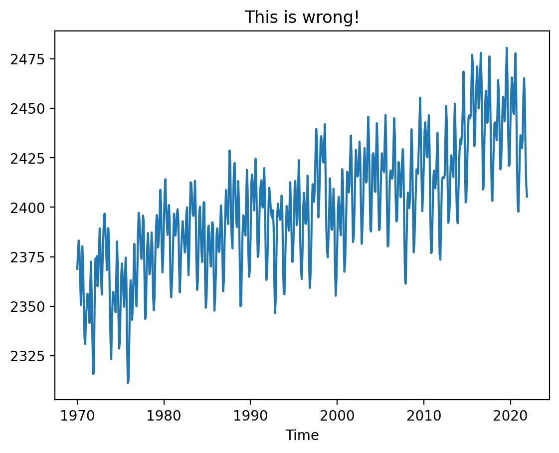
That would be wrong, however, because the denominator (weights.sum(dim='lat')) needs to be expanded to include the lon dimension and modified to account for the missing values (land points).

The weighted method

In general, weighted reductions on multidimensional arrays are complicated. To make it a bit easier, Xarray provides a mechanism for weighted reductions.

It does this by creating a special intermediate DataArrayWeighted object, to which different reduction operations can applied.

sst_weighted = ds.sst.weighted(weights)
sst_weighted

DataArrayWeighted with weights along dimensions: lat

Xarrays' computation methods (groupby, groupby_bins, rolling, coarsen, weighted) all return special objects that represent the basic underlying computation pattern. For e.g. `sst_weighted` above is a `DatasetWeighted` object that represents the weighting by `weights` of the data in `ds.sst`. It is usually helpful to save and reuse these objects for multiple operations (e.g. a mean and standard deviation calculation).

sst_weighted.mean(dim=("lon", "lat")).plot()
plt.title("Correct Global Mean SST");

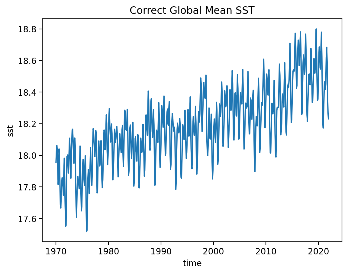
A handful of reductions have been implemented: mean, sum, std, var.