Advanced Indexing#
Learning Objectives#
Orthogonal vs. Pointwise (Vectorized) Indexing.
Pointwise indexing in Xarray to extract data at a collection of points.
Understand the difference between NumPy and Xarray indexing behavior.
Overview#
In the previous notebooks, we learned basic forms of indexing with Xarray, including positional and label-based indexing, datetime indexing, and nearest neighbor lookups. We also learned that indexing an Xarray DataArray directly works (mostly) like it does for NumPy arrays; however, Xarray indexing behavior deviates from NumPy when using multiple arrays for indexing, like arr[[0, 1], [0, 1]].
To better understand this difference, let’s take a look at an example of 2D 5x5 array:
array([[ 1,  2,  3,  4,  5],
       [ 6,  7,  8,  9, 10],
       [11, 12, 13, 14, 15],
       [16, 17, 18, 19, 20],
       [21, 22, 23, 24, 25]])
Now create a Xarray DataArray from this NumPy array:
import xarray as xr

da = xr.DataArray(np_array, dims=["x", "y"])
da
<xarray.DataArray (x: 5, y: 5)> Size: 200B
array([[ 1,  2,  3,  4,  5],
       [ 6,  7,  8,  9, 10],
       [11, 12, 13, 14, 15],
       [16, 17, 18, 19, 20],
       [21, 22, 23, 24, 25]])
Dimensions without coordinates: x, yNow, let’s see how the indexing behavior is different between NumPy array and Xarray DataArray when indexing with multiple arrays:
np_array[[0, 2, 4], [0, 2, 4]]
array([ 1, 13, 25])
da[[0, 2, 4], [0, 2, 4]]
<xarray.DataArray (x: 3, y: 3)> Size: 72B
array([[ 1,  3,  5],
       [11, 13, 15],
       [21, 23, 25]])
Dimensions without coordinates: x, yThe image below summarizes the difference between vectorized and orthogonal indexing for a 2D 5x5 NumPy array and Xarray DataArray:
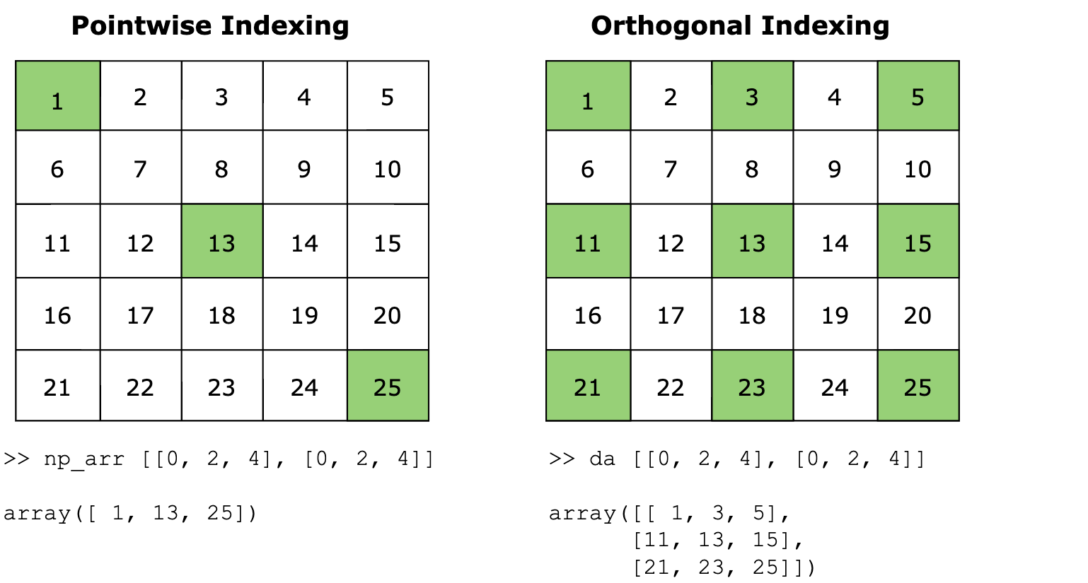
Pointwise or Vectorized indexing, shown on the left, selects specific elements at given coordinates, resulting in an array of those individual elements. In the example shown, the indices [0, 2, 4], [0, 2, 4] select the elements at positions (0, 0), (2, 2), and (4, 4), resulting in the values [1, 13, 25]. This is the default behavior of NumPy arrays.
In contrast, orthogonal indexing uses the same indices to select entire rows and columns, forming the Cartesian product of the specified indices. This method results in sub-arrays that include all combinations of the selected rows and columns. The example demonstrates this by selecting rows 0, 2, and 4 and columns 0, 2, and 4, resulting in a subarray containing [[1, 3, 5], [11, 13, 15], [21, 23, 25]]. This is Xarray DataArray’s default behavior.
The output of vectorized indexing is a 1D array, while the output of orthogonal indexing is a 3x3 array.
Tip
To Summarize:
Pointwise or vectorized indexing is a more general form of indexing that allows for arbitrary combinations of indexing arrays. This method of indexing is analogous to the broadcasting rules in NumPy, where the dimensions of the indexers are aligned and the result is determined by the shape of the indexers. This is the default behavior in NumPy.
Orthogonal or outer indexing allows for indexing along each dimension independently, treating the indexers as one-dimensional arrays. The principle of outer or orthogonal indexing is that the result mirrors the effect of independently indexing along each dimension with integer or boolean arrays, treating both the indexed and indexing arrays as one-dimensional. This method of indexing is analogous to vector indexing in programming languages like MATLAB, Fortran, and R, where each indexer component independently selects along its corresponding dimension. This is the default behavior in Xarray.
Orthogonal indexing with NumPy
While pointwise indexing is the default behavior in NumPy, you can achieve orthogonal indexing by using the np.ix_ function. This function constructs an open mesh from multiple arrays, allowing you to index along each dimension independently similar to Xarray indexing behavior. For example:
ixgrid = np.ix_([0, 2, 4], [0, 2, 4])
np_array[ixgrid]
Orthogonal Indexing in Xarray#
As explained earlier, when you use only integers, slices, or unlabeled arrays (arrays without dimension names, such as np.ndarray or list, but not DataArray) to index an Xarray DataArray, Xarray interprets these indexers orthogonally. This means it indexes along independent axes, rather than using NumPy’s broadcasting rules to vectorize the indexers.
In the example above we saw this behavior, but let’s see this behavior in action with a real dataset. Here we’ll use air temperature data from the National Center for Environmental Prediction:
import numpy as np
import xarray as xr

xr.set_options(display_expand_attrs=False)
np.set_printoptions(threshold=10, edgeitems=2)
%config InlineBackend.figure_format='retina'

ds = xr.tutorial.load_dataset("air_temperature")
da_air = ds.air
da_air
<xarray.DataArray 'air' (time: 2920, lat: 25, lon: 53)> Size: 31MB
array([[[241.2 , 242.5 , ..., 235.5 , 238.6 ],
        [243.8 , 244.5 , ..., 235.3 , 239.3 ],
        ...,
        [295.9 , 296.2 , ..., 295.9 , 295.2 ],
        [296.29, 296.79, ..., 296.79, 296.6 ]],

       [[242.1 , 242.7 , ..., 233.6 , 235.8 ],
        [243.6 , 244.1 , ..., 232.5 , 235.7 ],
        ...,
        [296.2 , 296.7 , ..., 295.5 , 295.1 ],
        [296.29, 297.2 , ..., 296.4 , 296.6 ]],

       ...,

       [[245.79, 244.79, ..., 243.99, 244.79],
        [249.89, 249.29, ..., 242.49, 244.29],
        ...,
        [296.29, 297.19, ..., 295.09, 294.39],
        [297.79, 298.39, ..., 295.49, 295.19]],

       [[245.09, 244.29, ..., 241.49, 241.79],
        [249.89, 249.29, ..., 240.29, 241.69],
        ...,
        [296.09, 296.89, ..., 295.69, 295.19],
        [297.69, 298.09, ..., 296.19, 295.69]]], shape=(2920, 25, 53))
Coordinates:
  * time     (time) datetime64[ns] 23kB 2013-01-01 ... 2014-12-31T18:00:00
  * lat      (lat) float32 100B 75.0 72.5 70.0 67.5 65.0 ... 22.5 20.0 17.5 15.0
  * lon      (lon) float32 212B 200.0 202.5 205.0 207.5 ... 325.0 327.5 330.0
Attributes: (11)selected_da = da_air.isel(time=0, lat=[2, 4, 10, 13], lon=[1, 6, 7]) # -- orthogonal indexing
selected_da
<xarray.DataArray 'air' (lat: 4, lon: 3)> Size: 96B
array([[249.8 , 243.1 , 242.39],
       [274.29, 271.79, 270.6 ],
       [277.4 , 280.6 , 280.9 ],
       [283.2 , 285.5 , 285.9 ]], shape=(4, 3))
Coordinates:
  * lat      (lat) float32 16B 70.0 65.0 50.0 42.5
  * lon      (lon) float32 12B 202.5 215.0 217.5
    time     datetime64[ns] 8B 2013-01-01
Attributes: (11)👆 Please note that the output shape in the example above is 4x3 because the latitude indexer selects 4 rows, and the longitude indexer selects 3 columns.
For more flexibility, you can supply DataArray() objects as indexers. Dimensions on resultant arrays are given by the ordered union of the indexers’ dimensions.
For example, in the example below we do orthogonal indexing using DataArray() objects.
target_lat = xr.DataArray([31, 41, 42, 42], dims="degrees_north")
target_lon = xr.DataArray([200, 201, 202, 205], dims="degrees_east")

da_air.sel(lat=target_lat, lon=target_lon, method="nearest")  # -- orthogonal indexing
<xarray.DataArray 'air' (time: 2920, degrees_north: 4, degrees_east: 4)> Size: 374kB
array([[[293.1 , 293.1 , 293.29, 293.29],
        [284.6 , 284.6 , 284.9 , 284.2 ],
        [282.79, 282.79, 283.2 , 282.6 ],
        [282.79, 282.79, 283.2 , 282.6 ]],

       [[293.2 , 293.2 , 293.9 , 294.2 ],
        [283.29, 283.29, 285.2 , 285.2 ],
        [281.4 , 281.4 , 282.79, 283.5 ],
        [281.4 , 281.4 , 282.79, 283.5 ]],

       ...,

       [[288.29, 288.29, 289.19, 290.79],
        [282.09, 282.09, 281.59, 282.39],
        [280.99, 280.99, 280.39, 280.59],
        [280.99, 280.99, 280.39, 280.59]],

       [[289.49, 289.49, 290.39, 291.59],
        [282.09, 282.09, 281.99, 283.09],
        [281.39, 281.39, 280.59, 280.99],
        [281.39, 281.39, 280.59, 280.99]]], shape=(2920, 4, 4))
Coordinates:
  * time     (time) datetime64[ns] 23kB 2013-01-01 ... 2014-12-31T18:00:00
    lat      (degrees_north) float32 16B 30.0 40.0 42.5 42.5
    lon      (degrees_east) float32 16B 200.0 200.0 202.5 205.0
Dimensions without coordinates: degrees_north, degrees_east
Attributes: (11)In the above example, you can see how the output shape is time x lats x lons. Please note that there are no shared dimensions between the indexers, so the output shape is the union of the dimensions of the indexers.
Attention
Please note that slices or sequences/arrays without named-dimensions are treated as if they have the same dimension which is indexed along.
For example:
da_air.sel(lat=[20, 30, 40], lon=target_lon, method="nearest")
<xarray.DataArray 'air' (time: 2920, lat: 3, degrees_east: 4)> Size: 280kB
array([[[296.6 , 296.6 , 296.2 , 296.4 ],
        [293.1 , 293.1 , 293.29, 293.29],
        [284.6 , 284.6 , 284.9 , 284.2 ]],

       [[296.4 , 296.4 , 295.9 , 296.2 ],
        [293.2 , 293.2 , 293.9 , 294.2 ],
        [283.29, 283.29, 285.2 , 285.2 ]],

       ...,

       [[293.69, 293.69, 293.89, 295.39],
        [288.29, 288.29, 289.19, 290.79],
        [282.09, 282.09, 281.59, 282.39]],

       [[293.79, 293.79, 293.69, 295.09],
        [289.49, 289.49, 290.39, 291.59],
        [282.09, 282.09, 281.99, 283.09]]], shape=(2920, 3, 4))
Coordinates:
  * time     (time) datetime64[ns] 23kB 2013-01-01 ... 2014-12-31T18:00:00
  * lat      (lat) float32 12B 20.0 30.0 40.0
    lon      (degrees_east) float32 16B 200.0 200.0 202.5 205.0
Dimensions without coordinates: degrees_east
Attributes: (11)But what if we’d like to find the nearest climate model grid cell to a collection of specified points (for example observation sites, or weather stations)?
Vectorized or Pointwise Indexing in Xarray#
Like NumPy and pandas, Xarray supports indexing many array elements at once in a vectorized manner.
Vectorized indexing or Pointwise Indexing using DataArrays() can be used to extract information from the nearest grid cells of interest, for example, the nearest climate model grid cells to a collection of specified observation tower data latitudes and longitudes.
Hint
To trigger vectorized indexing behavior, you will need to provide the selection dimensions with a new shared output dimension name. This means that the dimensions of both indexers must be the same, and the output will have the same dimension name as the indexers.
Let’s see how this works with an example:
A researcher wants to find the nearest climate model grid cell to a collection of observation sites. They have the latitude and longitude of the observation sites as following:
obs_lats = [31.81, 41.26, 22.59, 44.47, 28.57]

obs_lons = [200.16, 201.57, 305.54, 210.56, 226.59]
If the researcher use the lists to index the DataArray, they will get the orthogonal indexing behavior, which is not what they want.
da_air.sel(lat=obs_lats, lon=obs_lons, method="nearest") # -- orthogonal indexing
<xarray.DataArray 'air' (time: 2920, lat: 5, lon: 5)> Size: 584kB
array([[[290.2 , 290.79, ..., 293.1 , 290.  ],
        [282.79, 283.2 , ..., 282.2 , 283.7 ],
        ...,
        [280.  , 280.7 , ..., 280.29, 281.6 ],
        [293.79, 294.1 , ..., 295.4 , 290.4 ]],

       [[290.2 , 291.1 , ..., 292.4 , 291.1 ],
        [281.4 , 282.79, ..., 281.79, 284.  ],
        ...,
        [279.2 , 280.2 , ..., 280.1 , 282.1 ],
        [294.29, 294.79, ..., 295.29, 290.4 ]],

       ...,

       [[286.69, 287.89, ..., 291.39, 288.59],
        [280.99, 280.39, ..., 284.89, 283.49],
        ...,
        [279.69, 279.89, ..., 283.39, 281.29],
        [289.49, 290.39, ..., 293.89, 292.49]],

       [[287.59, 288.99, ..., 292.09, 288.49],
        [281.39, 280.59, ..., 284.99, 283.89],
        ...,
        [279.79, 279.29, ..., 283.59, 281.79],
        [289.79, 290.39, ..., 294.99, 292.39]]], shape=(2920, 5, 5))
Coordinates:
  * time     (time) datetime64[ns] 23kB 2013-01-01 ... 2014-12-31T18:00:00
  * lat      (lat) float32 20B 32.5 42.5 22.5 45.0 27.5
  * lon      (lon) float32 20B 200.0 202.5 305.0 210.0 227.5
Attributes: (11)To trigger the pointwise indexing, they need to create DataArray objects with the same dimension name, and then use them to index the DataArray.
For example, the code below first create DataArray objects for the latitude and longitude of the observation sites using a shared dimension name points, and then use them to index the DataArray air_temperature:
## latitudes of weather stations with a dimension of "points"
lat_points = xr.DataArray(obs_lats, dims="points")
lat_points
<xarray.DataArray (points: 5)> Size: 40B
array([31.81, 41.26, 22.59, 44.47, 28.57])
Dimensions without coordinates: points
## longitudes of weather stations with a dimension of "points"
lon_points = xr.DataArray(obs_lons, dims="points")
lon_points
<xarray.DataArray (points: 5)> Size: 40B
array([200.16, 201.57, 305.54, 210.56, 226.59])
Dimensions without coordinates: points
Now, retrieve data at the grid cells nearest to the target latitudes and longitudes (weather stations):
da_air.sel(lat=lat_points, lon=lon_points, method="nearest") # -- pointwise indexing
<xarray.DataArray 'air' (time: 2920, points: 5)> Size: 117kB
array([[290.2 , 283.2 , ..., 280.29, 290.4 ],
       [290.2 , 282.79, ..., 280.1 , 290.4 ],
       ...,
       [286.69, 280.39, ..., 283.39, 292.49],
       [287.59, 280.59, ..., 283.59, 292.39]], shape=(2920, 5))
Coordinates:
  * time     (time) datetime64[ns] 23kB 2013-01-01 ... 2014-12-31T18:00:00
    lat      (points) float32 20B 32.5 42.5 22.5 45.0 27.5
    lon      (points) float32 20B 200.0 202.5 305.0 210.0 227.5
Dimensions without coordinates: points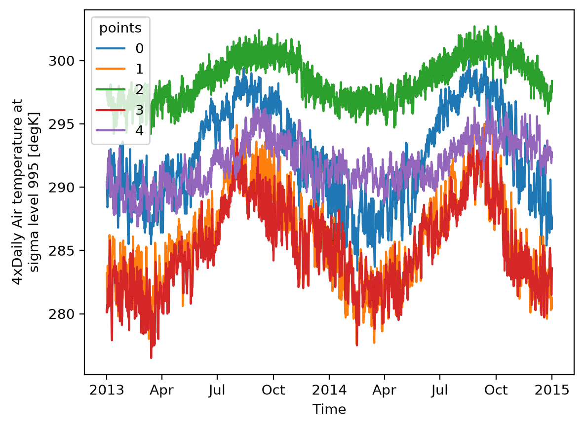
Attributes: (11)👆 Please notice how the shape of our DataArray is time x points, extracting time series for each weather stations.
da_air.sel(lat=lat_points, lon=lon_points, method="nearest").dims
('time', 'points')
Now, let’s plot the data for all stations.
da_air.sel(lat=lat_points, lon=lon_points, method="nearest").plot(x="time", hue="points");
Exercises#
Exercise
In the simple 2D 5x5 Xarray data array above, select the sub-array containing (0,4),(2,2),(4,0):
Solution
x_indices = np.array([0, 2, 4])
y_indices = np.array([4, 2, 0])

da_x = xr.DataArray(x_indices, dims="points")
da_y = xr.DataArray(y_indices, dims="points")

subset_da = da.sel(x=da_x, y=da_y)
subset_da