Re-organize InSAR ice velocity data#
This is an example of cleaning data accessed in netcdf format and preparing it for analysis.
The dataset we will use contains InSAR-derived ice velocity for 10 years over the Amundsen Sea Embayment in Antarctica. The data is downloaded from: https://nsidc.org/data/NSIDC-0545/versions/1 but this example uses only a subset of the full dataset.
Downloaded data is .hdr and .dat files for each year, and a .nc for all of the years together.
The .nc object is a dataset with dimensions x,y and data vars for each year. So for each year there are vx,vy,err vars. We’d like to re-organize this so that there are 3 variables (vx, vy and err) that exist along a time dimension.
Note
These steps were turned into a accessor/extension example, which can be viewed here.
ds = xr.tutorial.open_dataset("ASE_ice_velocity.nc")
ds
<xarray.Dataset> Size: 48MB
Dimensions:  (ny: 800, nx: 500)
Dimensions without coordinates: ny, nx
Data variables: (12/32)
    vx1996   (ny, nx) float32 2MB ...
    vy1996   (ny, nx) float32 2MB ...
    err1996  (ny, nx) float32 2MB ...
    vx2000   (ny, nx) float32 2MB ...
    vy2000   (ny, nx) float32 2MB ...
    err2000  (ny, nx) float32 2MB ...
    ...       ...
    err2011  (ny, nx) float32 2MB ...
    vx2012   (ny, nx) float32 2MB ...
    vy2012   (ny, nx) float32 2MB ...
    err2012  (ny, nx) float32 2MB ...
    xaxis    (nx) float32 2kB ...
    yaxis    (ny) float32 3kB ...
Attributes: (12/21)
    Title:                ASE Time Series - Ice Velocity
    Version:              1.0.0 (18Oct2013)
    nx:                   1707
    ny:                   2268
    Projection:                    Polar Stereographic South
    Ellipsoid:                      WGS-84
    ...                   ...
    Reference:                Mouginot J., B. Scheuchl and E. Rignot (2012), ...
    Notes_2:                    Please also include the following data set re...
    Data_citation:        NSIDC Citation Rignot, E., J. Mouginot, and B. Sche...
    More_information:     http://nsidc.org/data/nsidc-0545.html
    Notes_3:                       Data were processed at the Department of E...
Description: Created a spatial subset of original dataset. Selec...Take a look at the dataset:
ds
<xarray.Dataset> Size: 48MB
Dimensions:  (ny: 800, nx: 500)
Dimensions without coordinates: ny, nx
Data variables: (12/32)
    vx1996   (ny, nx) float32 2MB ...
    vy1996   (ny, nx) float32 2MB ...
    err1996  (ny, nx) float32 2MB ...
    vx2000   (ny, nx) float32 2MB ...
    vy2000   (ny, nx) float32 2MB ...
    err2000  (ny, nx) float32 2MB ...
    ...       ...
    err2011  (ny, nx) float32 2MB ...
    vx2012   (ny, nx) float32 2MB ...
    vy2012   (ny, nx) float32 2MB ...
    err2012  (ny, nx) float32 2MB ...
    xaxis    (nx) float32 2kB ...
    yaxis    (ny) float32 3kB ...
Attributes: (12/21)
    Title:                ASE Time Series - Ice Velocity
    Version:              1.0.0 (18Oct2013)
    nx:                   1707
    ny:                   2268
    Projection:                    Polar Stereographic South
    Ellipsoid:                      WGS-84
    ...                   ...
    Reference:                Mouginot J., B. Scheuchl and E. Rignot (2012), ...
    Notes_2:                    Please also include the following data set re...
    Data_citation:        NSIDC Citation Rignot, E., J. Mouginot, and B. Sche...
    More_information:     http://nsidc.org/data/nsidc-0545.html
    Notes_3:                       Data were processed at the Department of E...
Description: Created a spatial subset of original dataset. Selec...Check the projection:
ds.attrs["Projection"]
' Polar Stereographic South'
Currently the dimensions on the object are ny and nx but the object has no coordinates. If we look in the data_vars we can see there are two variables named xaxis and yaxis. It seems like these are the coordinate values that should exist along the nx and ny dimensions, respectively. Let’s confirm that they match the dimensions nx and ny in length and then assign them as coordinates:
800
500
/tmp/ipykernel_2873/3048788275.py:1: FutureWarning: The return type of `Dataset.dims` will be changed to return a set of dimension names in future, in order to be more consistent with `DataArray.dims`. To access a mapping from dimension names to lengths, please use `Dataset.sizes`.
  print(ds.dims["ny"])
/tmp/ipykernel_2873/3048788275.py:2: FutureWarning: The return type of `Dataset.dims` will be changed to return a set of dimension names in future, in order to be more consistent with `DataArray.dims`. To access a mapping from dimension names to lengths, please use `Dataset.sizes`.
  print(ds.dims["nx"])
We’ll assign the xaxis and yaxis vars to be coordinates, and drop them from the data_vars. We’ll first use swap_dims() to swap ny for yaxis and nx for xaxis.
ds = ds.swap_dims({"ny": "yaxis", "nx": "xaxis"})
ds
<xarray.Dataset> Size: 48MB
Dimensions:  (yaxis: 800, xaxis: 500)
Coordinates:
  * yaxis    (yaxis) float32 3kB -7.032e+05 -7.028e+05 ... -3.442e+05 -3.437e+05
  * xaxis    (xaxis) float32 2kB -1.581e+06 -1.581e+06 ... -1.357e+06 -1.357e+06
Data variables: (12/30)
    vx1996   (yaxis, xaxis) float32 2MB ...
    vy1996   (yaxis, xaxis) float32 2MB ...
    err1996  (yaxis, xaxis) float32 2MB ...
    vx2000   (yaxis, xaxis) float32 2MB ...
    vy2000   (yaxis, xaxis) float32 2MB ...
    err2000  (yaxis, xaxis) float32 2MB ...
    ...       ...
    vx2011   (yaxis, xaxis) float32 2MB ...
    vy2011   (yaxis, xaxis) float32 2MB ...
    err2011  (yaxis, xaxis) float32 2MB ...
    vx2012   (yaxis, xaxis) float32 2MB ...
    vy2012   (yaxis, xaxis) float32 2MB ...
    err2012  (yaxis, xaxis) float32 2MB ...
Attributes: (12/21)
    Title:                ASE Time Series - Ice Velocity
    Version:              1.0.0 (18Oct2013)
    nx:                   1707
    ny:                   2268
    Projection:                    Polar Stereographic South
    Ellipsoid:                      WGS-84
    ...                   ...
    Reference:                Mouginot J., B. Scheuchl and E. Rignot (2012), ...
    Notes_2:                    Please also include the following data set re...
    Data_citation:        NSIDC Citation Rignot, E., J. Mouginot, and B. Sche...
    More_information:     http://nsidc.org/data/nsidc-0545.html
    Notes_3:                       Data were processed at the Department of E...
Description: Created a spatial subset of original dataset. Selec...Rename yaxis and xaxis and drop the nx and ny coordinates:
ds = ds.rename({"xaxis": "x", "yaxis": "y"})
ds
<xarray.Dataset> Size: 48MB
Dimensions:  (y: 800, x: 500)
Coordinates:
  * y        (y) float32 3kB -7.032e+05 -7.028e+05 ... -3.442e+05 -3.437e+05
  * x        (x) float32 2kB -1.581e+06 -1.581e+06 ... -1.357e+06 -1.357e+06
Data variables: (12/30)
    vx1996   (y, x) float32 2MB ...
    vy1996   (y, x) float32 2MB ...
    err1996  (y, x) float32 2MB ...
    vx2000   (y, x) float32 2MB ...
    vy2000   (y, x) float32 2MB ...
    err2000  (y, x) float32 2MB ...
    ...       ...
    vx2011   (y, x) float32 2MB ...
    vy2011   (y, x) float32 2MB ...
    err2011  (y, x) float32 2MB ...
    vx2012   (y, x) float32 2MB ...
    vy2012   (y, x) float32 2MB ...
    err2012  (y, x) float32 2MB ...
Attributes: (12/21)
    Title:                ASE Time Series - Ice Velocity
    Version:              1.0.0 (18Oct2013)
    nx:                   1707
    ny:                   2268
    Projection:                    Polar Stereographic South
    Ellipsoid:                      WGS-84
    ...                   ...
    Reference:                Mouginot J., B. Scheuchl and E. Rignot (2012), ...
    Notes_2:                    Please also include the following data set re...
    Data_citation:        NSIDC Citation Rignot, E., J. Mouginot, and B. Sche...
    More_information:     http://nsidc.org/data/nsidc-0545.html
    Notes_3:                       Data were processed at the Department of E...
Description: Created a spatial subset of original dataset. Selec...Now we have x and y coordinates and 30 data variables. However, the data_vars are really only 3 unique variables that exist along a time dimension (with a length of 10).
We want to add a time dimension to the dataset and concatenate the data variables in each of the three groups together.
Start by making a few objects that we’ll use while we’re re-organizing. These are: a list of all the variables in the dataset (var_ls), a list of the years covered by the dataset that are currently stored in variable names (yr_ls) and then finally lists for each variable (vx_ls,vy_ls and err_ls). These are all of the variables in the original dataset that correspond with that main variable group (vx, vy or err).
Now we are going to group the dataset.data_vars into vx,vy, and err and prepare to concatenate them along the time dimension. We will perform the same operations for all three variables but we will demonstrate the process for the first variable in several steps, before showing the operation wrapped into one command for the other two variables. There is a great explanation of this kind of step here. At the end of this step, for vx, vy and err we will have a list of xr.DataArrays that all have a time dimension on the 0-axis.
In the cell below, we make a list of the xr.DataArrays in the original xr.Dataset that correspond to that variable.
da_vx_ls = [ds[var] for var in vx_ls]
You can see that da_vx_ls is a list object with a length of 10, and each element of the list is a xr.DataArray corresponding to vx vars in the original xr.Dataset
Object type:  <class 'list'>
Object length:  10
<xarray.DataArray 'vx1996' (y: 800, x: 500)> Size: 2MB
[400000 values with dtype=float32]
Coordinates:
  * y        (y) float32 3kB -7.032e+05 -7.028e+05 ... -3.442e+05 -3.437e+05
  * x        (x) float32 2kB -1.581e+06 -1.581e+06 ... -1.357e+06 -1.357e+06
Attributes:
    Content:  Ice velocity in x direction
Units: meter/yearnext, we will add a time dimension to every element of da_vx_ls:
Now you can see that each list element is an xr.DataArray as before, but that there is now a time dimension.
da_vx_ls[0]
<xarray.DataArray 'vx1996' (time: 1, y: 800, x: 500)> Size: 2MB
array([[[         nan,          nan,          nan, ...,          nan,
                  nan,          nan],
        [         nan,          nan,          nan, ...,          nan,
                  nan,          nan],
        [         nan,          nan,          nan, ...,          nan,
                  nan,          nan],
        ...,
        [  9.245862  ,  18.962032  ,  10.641378  , ..., -55.529568  ,
         -55.257446  , -55.041527  ],
        [  8.298822  ,  15.363108  ,   0.68973774, ..., -55.069824  ,
         -54.748978  , -54.98798   ],
        [  9.707195  ,  10.79028   ,  -6.217383  , ..., -54.61062   ,
         -55.119358  , -54.695946  ]]], shape=(1, 800, 500), dtype=float32)
Coordinates:
  * y        (y) float32 3kB -7.032e+05 -7.028e+05 ... -3.442e+05 -3.437e+05
  * x        (x) float32 2kB -1.581e+06 -1.581e+06 ... -1.357e+06 -1.357e+06
Dimensions without coordinates: time
Attributes:
    Content:  Ice velocity in x direction
Units: meter/yearAssign time as a coordinate to each xr.DataArray in the list:
<xarray.DataArray 'vx1996' (time: 1, y: 800, x: 500)> Size: 2MB
array([[[         nan,          nan,          nan, ...,          nan,
                  nan,          nan],
        [         nan,          nan,          nan, ...,          nan,
                  nan,          nan],
        [         nan,          nan,          nan, ...,          nan,
                  nan,          nan],
        ...,
        [  9.245862  ,  18.962032  ,  10.641378  , ..., -55.529568  ,
         -55.257446  , -55.041527  ],
        [  8.298822  ,  15.363108  ,   0.68973774, ..., -55.069824  ,
         -54.748978  , -54.98798   ],
        [  9.707195  ,  10.79028   ,  -6.217383  , ..., -54.61062   ,
         -55.119358  , -54.695946  ]]], shape=(1, 800, 500), dtype=float32)
Coordinates:
* time (time) int64 8B 1996
* y (y) float32 3kB -7.032e+05 -7.028e+05 ... -3.442e+05 -3.437e+05
* x (x) float32 2kB -1.581e+06 -1.581e+06 ... -1.357e+06 -1.357e+06
Attributes:
Content: Ice velocity in x direction
Units: meter/yearTime is now a coordinate as well as a dimension and the coordinate value corresponds to the element-order of the list, ie. the first (0-place) element of da_vx_ls_test is the xr.DataArray containing the vx1996 variable, and the time coord is 0. In the second (1-place) element, the xr.DataArray is called vx2000 and the time coord is 1.
Finally, we will rename the xr.DataArrays to reflect just the variable name, rather than the year, because that is now referenced in the time coordinate.
da_vx_ls[2]
<xarray.DataArray 'vx' (time: 1, y: 800, x: 500)> Size: 2MB
array([[[      nan,       nan,       nan, ...,       nan,       nan,
               nan],
        [      nan,       nan,       nan, ...,       nan,       nan,
               nan],
        [      nan,       nan,       nan, ...,       nan,       nan,
               nan],
        ...,
        [38.909744, 40.761253, 19.25432 , ...,       nan,       nan,
               nan],
        [38.70002 , 39.267914, 11.182553, ...,       nan,       nan,
               nan],
        [39.49789 , 42.261513, 16.20535 , ...,       nan,       nan,
               nan]]], shape=(1, 800, 500), dtype=float32)
Coordinates:
  * time     (time) int64 8B 2002
  * y        (y) float32 3kB -7.032e+05 -7.028e+05 ... -3.442e+05 -3.437e+05
  * x        (x) float32 2kB -1.581e+06 -1.581e+06 ... -1.357e+06 -1.357e+06
Attributes:
    Content:  Ice velocity in x direction
Units: meter/yearNow we have a list of xr.DataArrays for the vx data variable where each xr.DataArray has a time dimension and coordinates along the time dimension. This list is ready to be concatenated along the time dimension.
First, we will perform the same steps for the other two data variables (vy and err) before concatenating all three along the time dimension and merging into one xr.Dataset. For vy and err, we will combine the steps followed for vx into one operation. Note one other difference between the workflow for vx and the workflow for vy and err: rather than assigning coordinate values using the assign_coords() function, we do this within the expand_dims() function, where a time dimension is added as well as coordinate values for the dimension ([int(var[-4:])]).
Once we have these lists, we will concatenate them together to a single xr.DataArray with x,y and time dimensions. In the above step, when we create the time dimension we assign a stand-in for the time coordinate. In the cell below, we’ll use the yr_ls object that we created that is a list whose elements are time-aware objects corresponding to the time coordinates (originally in the variable names). The final line in the cell below merges the three xr.DataArrays on the common time dimension that they now share, so we have a xr.Dataset with x,y and time dimensions and vx, vy and err variables.
ds_merge
<xarray.Dataset> Size: 48MB
Dimensions:  (x: 500, y: 800, time: 10)
Coordinates:
  * x        (x) float32 2kB -1.581e+06 -1.581e+06 ... -1.357e+06 -1.357e+06
  * y        (y) float32 3kB -7.032e+05 -7.028e+05 ... -3.442e+05 -3.437e+05
  * time     (time) int64 80B 1996 2000 2002 2006 2007 2008 2009 2010 2011 2012
Data variables:
    vx       (time, y, x) float32 16MB nan nan nan nan nan ... nan nan nan nan
    vy       (time, y, x) float32 16MB nan nan nan nan nan ... nan nan nan nan
    err      (time, y, x) float32 16MB nan nan nan nan nan ... nan nan nan nan
Attributes:
    Content:  Ice velocity in x direction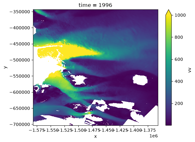
Units: meter/yearWe’ll add a variable that is magnitude of velocity as well
ds_merge["vv"] = np.sqrt((ds_merge.vx**2) + (ds_merge.vy**2))
ds_merge.vv.isel(time=0).plot(vmax=1000)
<matplotlib.collections.QuadMesh at 0x7f9c2580ea50>
and add the attrs of the original object to our new object, ds_full
ds_merge.attrs = ds.attrs
ds_merge
<xarray.Dataset> Size: 64MB
Dimensions:  (x: 500, y: 800, time: 10)
Coordinates:
  * x        (x) float32 2kB -1.581e+06 -1.581e+06 ... -1.357e+06 -1.357e+06
  * y        (y) float32 3kB -7.032e+05 -7.028e+05 ... -3.442e+05 -3.437e+05
  * time     (time) int64 80B 1996 2000 2002 2006 2007 2008 2009 2010 2011 2012
Data variables:
    vx       (time, y, x) float32 16MB nan nan nan nan nan ... nan nan nan nan
    vy       (time, y, x) float32 16MB nan nan nan nan nan ... nan nan nan nan
    err      (time, y, x) float32 16MB nan nan nan nan nan ... nan nan nan nan
    vv       (time, y, x) float32 16MB nan nan nan nan nan ... nan nan nan nan
Attributes: (12/21)
    Title:                ASE Time Series - Ice Velocity
    Version:              1.0.0 (18Oct2013)
    nx:                   1707
    ny:                   2268
    Projection:                    Polar Stereographic South
    Ellipsoid:                      WGS-84
    ...                   ...
    Reference:                Mouginot J., B. Scheuchl and E. Rignot (2012), ...
    Notes_2:                    Please also include the following data set re...
    Data_citation:        NSIDC Citation Rignot, E., J. Mouginot, and B. Sche...
    More_information:     http://nsidc.org/data/nsidc-0545.html
    Notes_3:                       Data were processed at the Department of E...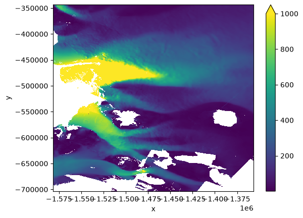
Description: Created a spatial subset of original dataset. Selec...Checking against original version to make sure it’s the same:
np.sqrt((ds.vx1996**2) + (ds.vy1996**2)).plot(vmax=1000)
<matplotlib.collections.QuadMesh at 0x7f9c256e6490>
We can also use xr.DataArray.equals function to test if two xr.DataArrays are identical to one another. More information here.
ds_merge["vx"].sel(time=1996, drop=True).equals(ds.vx1996)
True