Windowed Computations#
Xarray has built-in support for windowed operations:
In this notebook, we’ll learn to
Compute rolling, or sliding window, means along one or more dimensions.
Compute block averages along a dimension.
Use
constructto reshape arrays so that a new dimension provides windowed views to the data.
import matplotlib.pyplot as plt
import numpy as np
import xarray as xr

np.set_printoptions(threshold=10, edgeitems=2)
xr.set_options(display_expand_data=False)

%config InlineBackend.figure_format='retina'
ds = xr.tutorial.load_dataset("ersstv5")
ds
<xarray.Dataset> Size: 40MB
Dimensions:    (time: 624, nbnds: 2, lat: 89, lon: 180)
Coordinates:
  * time       (time) datetime64[ns] 5kB 1970-01-01 1970-02-01 ... 2021-12-01
  * lat        (lat) float32 356B 88.0 86.0 84.0 82.0 ... -84.0 -86.0 -88.0
  * lon        (lon) float32 720B 0.0 2.0 4.0 6.0 ... 352.0 354.0 356.0 358.0
Dimensions without coordinates: nbnds
Data variables:
    time_bnds  (time, nbnds) float64 10kB 9.969e+36 9.969e+36 ... 9.969e+36
    sst        (time, lat, lon) float32 40MB -1.8 -1.8 -1.8 -1.8 ... nan nan nan
Attributes: (12/37)
    climatology:               Climatology is based on 1971-2000 SST, Xue, Y....
    description:               In situ data: ICOADS2.5 before 2007 and NCEP i...
    keywords_vocabulary:       NASA Global Change Master Directory (GCMD) Sci...
    keywords:                  Earth Science > Oceans > Ocean Temperature > S...
    instrument:                Conventional thermometers
    source_comment:            SSTs were observed by conventional thermometer...
    ...                        ...
    creator_url_original:      https://www.ncei.noaa.gov
    license:                   No constraints on data access or use
    comment:                   SSTs were observed by conventional thermometer...
    summary:                   ERSST.v5 is developed based on v4 after revisi...
    dataset_title:             NOAA Extended Reconstructed SST V5
data_modified: 2022-06-07Rolling or moving windows#
Rolling window operations
can be applied along any dimension, or along multiple dimensions.
returns object of same shape as input
pads with NaNs to make (2) possible
Again, all common reduction operations are available
rolling = ds.rolling(time=12, center=True)
rolling
DatasetRolling [time->12(center)]
Tip
Xarrays’ computation methods (groupby, groupby_bins, rolling, coarsen, weighted) all return special objects that represent the basic underlying computation pattern. For e.g. rolling above is a DatasetRolling object that represents 12-point rolling windows of the data in ds . It is usually helpful to save and reuse these objects for multiple operations (e.g. a mean and standard deviation calculation).
ds_rolling = rolling.mean()
ds_rolling
<xarray.Dataset> Size: 40MB
Dimensions:    (time: 624, nbnds: 2, lat: 89, lon: 180)
Coordinates:
  * time       (time) datetime64[ns] 5kB 1970-01-01 1970-02-01 ... 2021-12-01
  * lat        (lat) float32 356B 88.0 86.0 84.0 82.0 ... -84.0 -86.0 -88.0
  * lon        (lon) float32 720B 0.0 2.0 4.0 6.0 ... 352.0 354.0 356.0 358.0
Dimensions without coordinates: nbnds
Data variables:
    time_bnds  (time, nbnds) float64 10kB nan nan nan nan ... nan nan nan nan
    sst        (time, lat, lon) float32 40MB nan nan nan nan ... nan nan nan nan
Attributes: (12/37)
    climatology:               Climatology is based on 1971-2000 SST, Xue, Y....
    description:               In situ data: ICOADS2.5 before 2007 and NCEP i...
    keywords_vocabulary:       NASA Global Change Master Directory (GCMD) Sci...
    keywords:                  Earth Science > Oceans > Ocean Temperature > S...
    instrument:                Conventional thermometers
    source_comment:            SSTs were observed by conventional thermometer...
    ...                        ...
    creator_url_original:      https://www.ncei.noaa.gov
    license:                   No constraints on data access or use
    comment:                   SSTs were observed by conventional thermometer...
    summary:                   ERSST.v5 is developed based on v4 after revisi...
    dataset_title:             NOAA Extended Reconstructed SST V5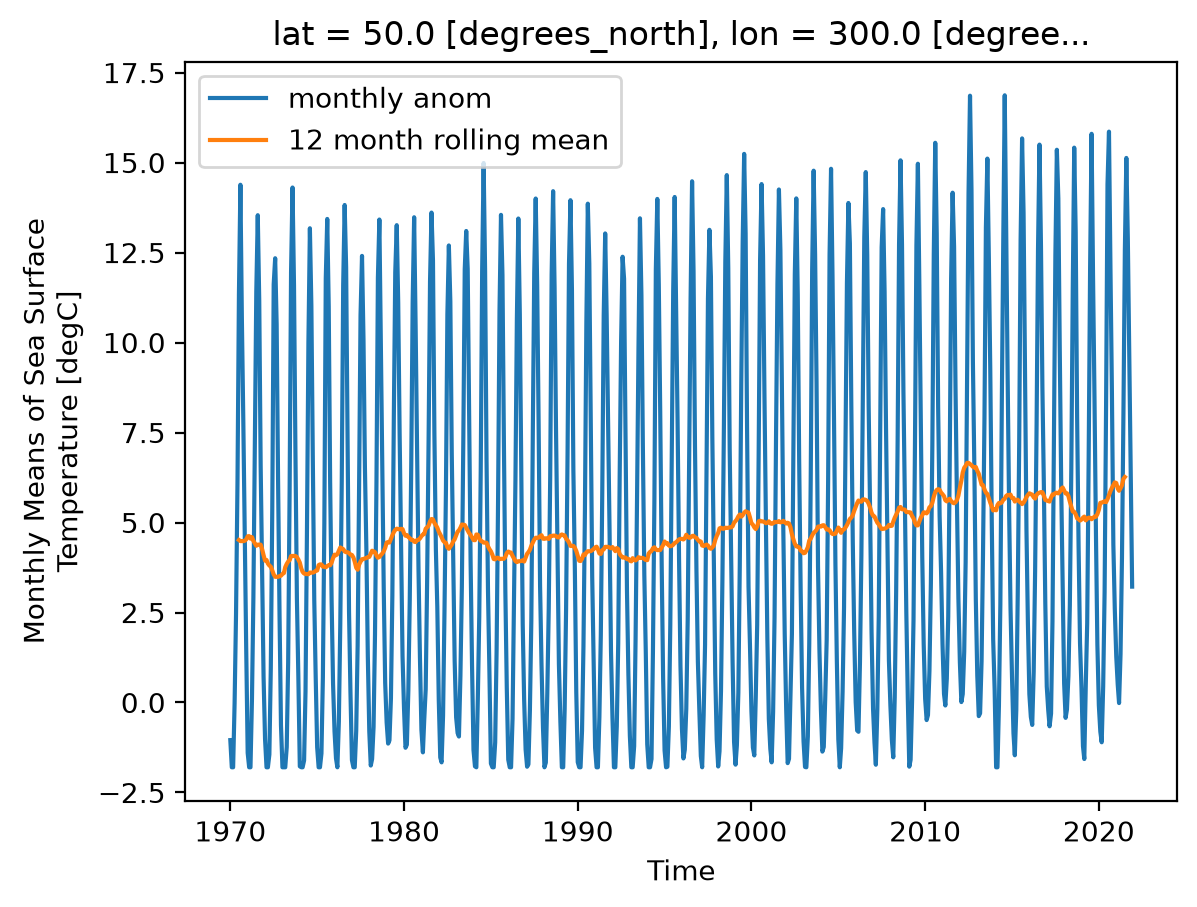
data_modified: 2022-06-07ds.sst.sel(lon=300, lat=50).plot(label="monthly anom")
ds_rolling.sst.sel(lon=300, lat=50).plot(label="12 month rolling mean")
plt.legend()
<matplotlib.legend.Legend at 0x7feae8f22cf0>
We can apply rolling mean along multiple dimensions as a 2D smoother in (lat, lon). Here is an example of a 5-point running mean applied along both the lat and lon dimensions
extract = ds.sst.isel(time=0)
smoothed = extract.rolling(lon=5, lat=5, center=True).mean()

f, ax = plt.subplots(2, 1, sharex=True, sharey=True)
extract.plot(ax=ax[0], robust=True)
smoothed.plot(ax=ax[1], robust=True)
f.set_size_inches((10, 7))
plt.tight_layout()
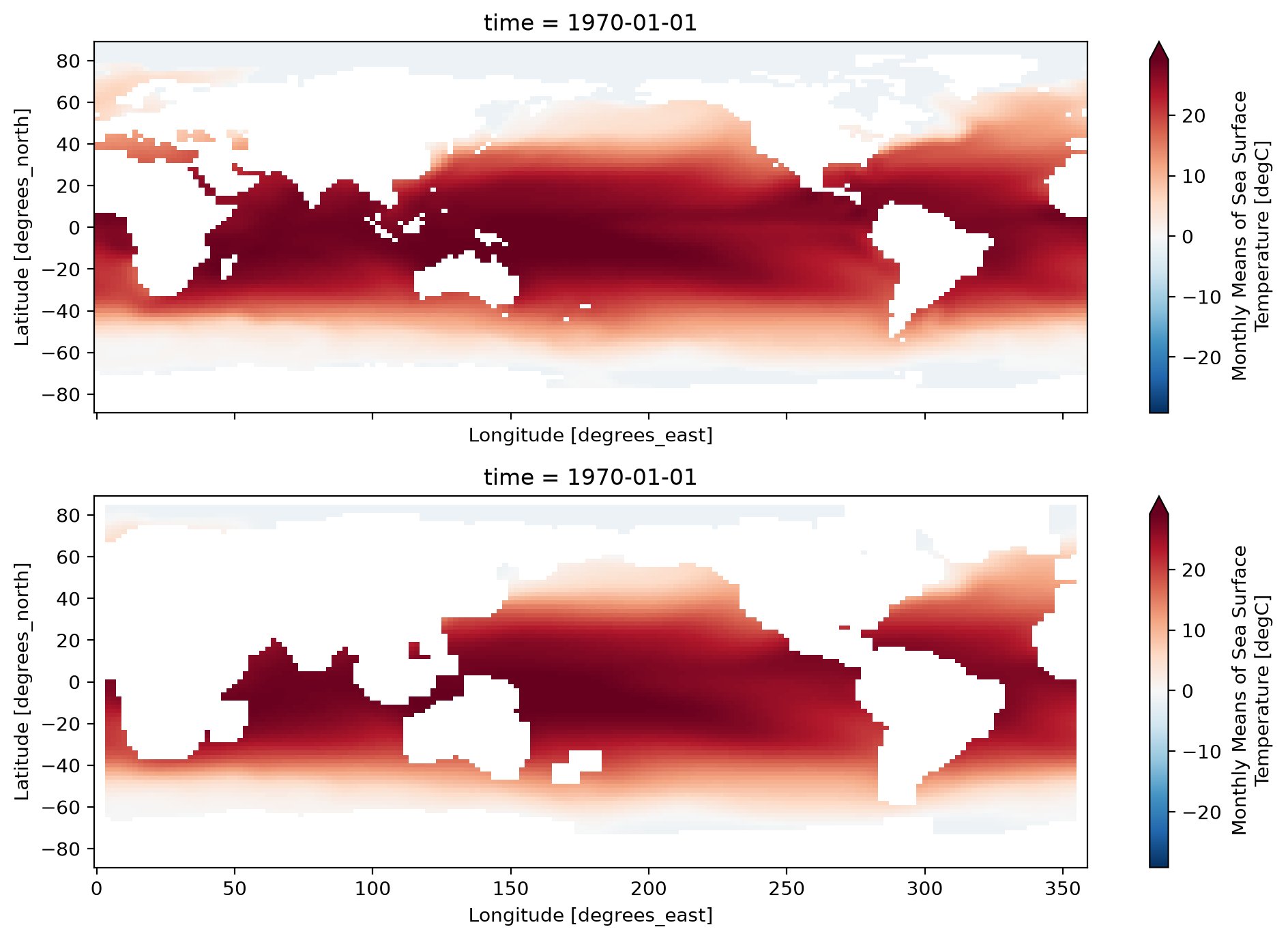
Note the addition of NaNs at the data boundaries and near continental boundaries.
Custom reductions#
While common reductions are implemented by default, sometimes it is useful to apply our own windowed operations. For these uses, Xarray provides the construct methods for DataArray.rolling and Dataset.rolling.
For rolling over a dimension time with a window size N, construct adds a new dimension (with user-provided name) of size N.
We illustrate with a simple example array:
simple = xr.DataArray(np.arange(10), dims="time", coords={"time": np.arange(10)})
simple
<xarray.DataArray (time: 10)> Size: 80B
0 1 2 3 4 5 6 7 8 9
Coordinates:
  * time     (time) int64 80B 0 1 2 3 4 5 6 7 8 9
We call construct and provide a name for the new dimension: window
# adds a new dimension "window"
simple.rolling(time=5, center=True).construct("window")
<xarray.DataArray (time: 10, window: 5)> Size: 400B
nan nan 0.0 1.0 2.0 nan 0.0 1.0 2.0 3.0 ... 7.0 8.0 9.0 nan 7.0 8.0 9.0 nan nan
Coordinates:
  * time     (time) int64 80B 0 1 2 3 4 5 6 7 8 9
Dimensions without coordinates: window
Exercise
Illustrate the difference between center=True and center=False for rolling by looking at the construct-ed array.
Solution
display("center=True")
display(simple.rolling(time=5, center=True).construct("window"))

display("center=False")
display(simple.rolling(time=5, center=False).construct("window"))
Coarsening#
coarsen does something similar to rolling, but allows us to work with discrete non-overlapping blocks of data.
You will need to specify boundary if the length of the dimension is not a multiple of the window size (“block size”). You can choose to
trimthe excess valuespadwith NaNs
Again, all standard reductions are implemented.
coarse = ds.coarsen(lon=5, lat=5)
coarse
DatasetCoarsen [windows->{'lon': 5, 'lat': 5},side->left]
Xarrays’ computation methods (groupby, groupby_bins, rolling, coarsen, weighted) all return special objects that represent the basic underlying computation pattern. For e.g. coarse above is a DatasetCoarsen object that represents 5-point windows along lat, lon of the data in ds. It is usually helpful to save and reuse these objects for multiple operations (e.g. a mean and standard deviation calculation).
# we expect an error here because lat has size 89, which is not divisible by block size 5
coarse.mean()
---------------------------------------------------------------------------
ValueError                                Traceback (most recent call last)
Cell In[10], line 2
      1 # we expect an error here because lat has size 89, which is not divisible by block size 5
----> 2 coarse.mean()

File ~/work/xarray-tutorial/xarray-tutorial/.pixi/envs/default/lib/python3.14/site-packages/xarray/computation/rolling.py:1339, in DatasetCoarsen._reduce_method.<locals>.wrapped_func(self, keep_attrs, **kwargs)
   1337 reduced = {}
   1338 for key, da in self.obj.data_vars.items():
-> 1339     reduced[key] = da.variable.coarsen(
   1340         self.windows,
   1341         func,
   1342         self.boundary,
   1343         self.side,
   1344         keep_attrs=keep_attrs,
   1345         **kwargs,
   1346     )
   1348 coords = {}
   1349 for c, v in self.obj.coords.items():
   1350     # variable.coarsen returns variables not containing the window dims
   1351     # unchanged (maybe removes attrs)

File ~/work/xarray-tutorial/xarray-tutorial/.pixi/envs/default/lib/python3.14/site-packages/xarray/core/variable.py:2268, in Variable.coarsen(self, windows, func, boundary, side, keep_attrs, **kwargs)
   2265 if not windows:
   2266     return self._replace(attrs=_attrs)
-> 2268 reshaped, axes = self.coarsen_reshape(windows, boundary, side)
   2269 if isinstance(func, str):
   2270     name = func

File ~/work/xarray-tutorial/xarray-tutorial/.pixi/envs/default/lib/python3.14/site-packages/xarray/core/variable.py:2305, in Variable.coarsen_reshape(self, windows, boundary, side)
   2303 if boundary[d] == "exact":
   2304     if n * window != size:
-> 2305         raise ValueError(
   2306             f"Could not coarsen a dimension of size {size} with "
   2307             f"window {window} and boundary='exact'. Try a different 'boundary' option."
   2308         )
   2309 elif boundary[d] == "trim":
   2310     if side[d] == "left":

ValueError: Could not coarsen a dimension of size 89 with window 5 and boundary='exact'. Try a different 'boundary' option.
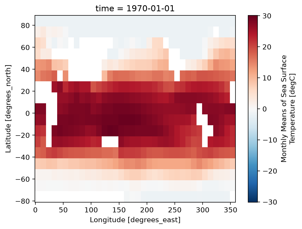
coarse = ds.coarsen(lat=5, lon=5, boundary="trim").mean()
coarse
<xarray.Dataset> Size: 2MB
Dimensions:    (time: 624, nbnds: 2, lat: 17, lon: 36)
Coordinates:
  * time       (time) datetime64[ns] 5kB 1970-01-01 1970-02-01 ... 2021-12-01
  * lat        (lat) float32 68B 84.0 74.0 64.0 54.0 ... -46.0 -56.0 -66.0 -76.0
  * lon        (lon) float32 144B 4.0 14.0 24.0 34.0 ... 324.0 334.0 344.0 354.0
Dimensions without coordinates: nbnds
Data variables:
    time_bnds  (time, nbnds) float64 10kB 9.969e+36 9.969e+36 ... 9.969e+36
    sst        (time, lat, lon) float32 2MB -1.757 -1.78 -1.8 ... -1.685 nan
Attributes: (12/37)
    climatology:               Climatology is based on 1971-2000 SST, Xue, Y....
    description:               In situ data: ICOADS2.5 before 2007 and NCEP i...
    keywords_vocabulary:       NASA Global Change Master Directory (GCMD) Sci...
    keywords:                  Earth Science > Oceans > Ocean Temperature > S...
    instrument:                Conventional thermometers
    source_comment:            SSTs were observed by conventional thermometer...
    ...                        ...
    creator_url_original:      https://www.ncei.noaa.gov
    license:                   No constraints on data access or use
    comment:                   SSTs were observed by conventional thermometer...
    summary:                   ERSST.v5 is developed based on v4 after revisi...
    dataset_title:             NOAA Extended Reconstructed SST V5
data_modified: 2022-06-07coarse.sst.isel(time=0).plot();
Custom reductions#
Like rolling, coarsen also provides a construct method for custom block operations.
Tip
coarsen.construct is a handy way to reshape Xarray objects.
Consider a “monthly” 1D timeseries. This simple example has one value per month for 2 years
<xarray.DataArray (time: 24)> Size: 192B
1 2 3 4 5 6 7 8 9 10 11 12 1 2 3 4 5 6 7 8 9 10 11 12
Coordinates:
  * time     (time) int64 192B 1 2 3 4 5 6 7 8 9 ... 16 17 18 19 20 21 22 23 24
Now we reshape to get one new dimension year of size 12.
# break "time" into two new dimensions: "year", "month"
months.coarsen(time=12).construct(time=("year", "month"))
<xarray.DataArray (year: 2, month: 12)> Size: 192B
1 2 3 4 5 6 7 8 9 10 11 12 1 2 3 4 5 6 7 8 9 10 11 12
Coordinates:
    time     (year, month) int64 192B 1 2 3 4 5 6 7 8 ... 18 19 20 21 22 23 24
Dimensions without coordinates: year, monthExercise
Imagine the array months was one element shorter. Use boundary="pad" and the side kwarg to reshape months.isel(time=slice(1, None)) to a 2D DataArray with the following values:
array([[nan,  2.,  3.,  4.,  5.,  6.,  7.,  8.,  9., 10., 11., 12.],
       [ 1.,  2.,  3.,  4.,  5.,  6.,  7.,  8.,  9., 10., 11., 12.]])
Solution
months.isel(time=slice(1, None)).coarsen({"time": 12}, boundary="pad", side="right").construct(
    time=("year", "month")
)
Note that coarsen pads with NaNs. For more control over padding, use
DataArray.pad explicitly.
Going further#
Follow the tutorial on high-level computational patterns