Parallel computing with Dask#
This notebook demonstrates one of Xarray’s most powerful features: the ability to wrap dask arrays and allow users to seamlessly execute analysis code in parallel.
By the end of this notebook, you will:
Xarray DataArrays and Datasets are “dask collections” i.e. you can execute top-level dask functions such as
dask.visualize(xarray_object)Learn that all xarray built-in operations can transparently use dask
Important
Using Dask does not always make your computations run faster!*
Performance will depend on the computational infrastructure you’re using (for example, how many CPU cores), how the data you’re working with is structured and stored, and the algorithms and code you’re running. Be sure to review the Dask best-practices if you’re new to Dask!
What is Dask#
When we talk about Xarray + Dask, we are usually talking about two things:
dask.arrayas a drop-in replacement for numpy arraysA “scheduler” that actually runs computations on dask arrays (commonly distributed)
Introduction to dask.array#
Dask Array implements a subset of the NumPy ndarray interface using blocked algorithms, cutting up the large array into many small arrays (blocks or chunks). This lets us compute on arrays larger than memory using all of our cores. We coordinate these blocked algorithms using Dask graphs.

import dask
import dask.array

dasky = dask.array.ones((10, 5), chunks=(2, 2))
dasky
|
||||||||||||||||
Why dask.array#
Use parallel resources to speed up computation
Work with datasets bigger than RAM (“out-of-core”)
“dask lets you scale from memory-sized datasets to disk-sized datasets”
dask is lazy#
Operations are not computed until you explicitly request them.
dasky.mean(axis=-1)
|
||||||||||||||||
So what did dask do when you called .mean? It added that operation to the “graph” or a blueprint of operations to execute later.
dask.visualize(dasky.mean(axis=-1))
dasky.mean(axis=-1).compute()
array([1., 1., 1., 1., 1., 1., 1., 1., 1., 1.])
More#
See the dask.array tutorial
Dask + Xarray#
Remember that Xarray can wrap many different array types. So Xarray can wrap dask arrays too.
We use Xarray to enable using our metadata to express our analysis.
Creating dask-backed Xarray objects#
The chunks argument to both open_dataset and open_mfdataset allow you to
read datasets as dask arrays.
%xmode minimal

import numpy as np
import xarray as xr

# limit the amount of information printed to screen
xr.set_options(display_expand_data=False)
np.set_printoptions(threshold=10, edgeitems=2)
Exception reporting mode: Minimal
ds = xr.tutorial.open_dataset("air_temperature")
ds.air
<xarray.DataArray 'air' (time: 2920, lat: 25, lon: 53)> Size: 31MB
[3869000 values with dtype=float64]
Coordinates:
  * time     (time) datetime64[ns] 23kB 2013-01-01 ... 2014-12-31T18:00:00
  * lat      (lat) float32 100B 75.0 72.5 70.0 67.5 65.0 ... 22.5 20.0 17.5 15.0
  * lon      (lon) float32 212B 200.0 202.5 205.0 207.5 ... 325.0 327.5 330.0
Attributes:
    long_name:     4xDaily Air temperature at sigma level 995
    units:         degK
    precision:     2
    GRIB_id:       11
    GRIB_name:     TMP
    var_desc:      Air temperature
    dataset:       NMC Reanalysis
    level_desc:    Surface
    statistic:     Individual Obs
    parent_stat:   Other
actual_range: [185.16 322.1 ]ds = xr.tutorial.open_dataset(
"air_temperature",
chunks={ # this tells xarray to open the dataset as a dask array
"lat": "auto",
"lon": 25,
"time": -1,
},
)
ds
<xarray.Dataset> Size: 31MB
Dimensions:  (time: 2920, lat: 25, lon: 53)
Coordinates:
  * time     (time) datetime64[ns] 23kB 2013-01-01 ... 2014-12-31T18:00:00
  * lat      (lat) float32 100B 75.0 72.5 70.0 67.5 65.0 ... 22.5 20.0 17.5 15.0
  * lon      (lon) float32 212B 200.0 202.5 205.0 207.5 ... 325.0 327.5 330.0
Data variables:
    air      (time, lat, lon) float64 31MB dask.array<chunksize=(2920, 25, 25), meta=np.ndarray>
Attributes:
    Conventions:  COARDS
    title:        4x daily NMC reanalysis (1948)
    description:  Data is from NMC initialized reanalysis\n(4x/day).  These a...
    platform:     Model
references: http://www.esrl.noaa.gov/psd/data/gridded/data.ncep.reanaly...The representation (“repr” in Python parlance) for the air DataArray shows the very nice HTML dask array repr. You can access the underlying chunk sizes using .chunks:
ds.air.chunks
((2920,), (25,), (25, 25, 3))
ds
<xarray.Dataset> Size: 31MB
Dimensions:  (time: 2920, lat: 25, lon: 53)
Coordinates:
  * time     (time) datetime64[ns] 23kB 2013-01-01 ... 2014-12-31T18:00:00
  * lat      (lat) float32 100B 75.0 72.5 70.0 67.5 65.0 ... 22.5 20.0 17.5 15.0
  * lon      (lon) float32 212B 200.0 202.5 205.0 207.5 ... 325.0 327.5 330.0
Data variables:
    air      (time, lat, lon) float64 31MB dask.array<chunksize=(2920, 25, 25), meta=np.ndarray>
Attributes:
    Conventions:  COARDS
    title:        4x daily NMC reanalysis (1948)
    description:  Data is from NMC initialized reanalysis\n(4x/day).  These a...
    platform:     Model
references: http://www.esrl.noaa.gov/psd/data/gridded/data.ncep.reanaly...Tip
All variables in a Dataset need not have the same chunk size along
common dimensions.
Extracting underlying data#
There are two ways to pull out the underlying array object in an xarray object.
.to_numpyor.valueswill always return a NumPy array. For dask-backed xarray objects, this means that compute will always be called.datawill return a Dask array
Tip
Use to_numpy or as_numpy instead of .values so that your code generalizes to other array types (like CuPy arrays, sparse arrays)
ds.air.data # dask array, not numpy
|
||||||||||||||||
ds.air.as_numpy().data ## numpy array
array([[[241.2 , 242.5 , ..., 235.5 , 238.6 ],
        [243.8 , 244.5 , ..., 235.3 , 239.3 ],
        ...,
        [295.9 , 296.2 , ..., 295.9 , 295.2 ],
        [296.29, 296.79, ..., 296.79, 296.6 ]],

       [[242.1 , 242.7 , ..., 233.6 , 235.8 ],
        [243.6 , 244.1 , ..., 232.5 , 235.7 ],
        ...,
        [296.2 , 296.7 , ..., 295.5 , 295.1 ],
        [296.29, 297.2 , ..., 296.4 , 296.6 ]],

       ...,

       [[245.79, 244.79, ..., 243.99, 244.79],
        [249.89, 249.29, ..., 242.49, 244.29],
        ...,
        [296.29, 297.19, ..., 295.09, 294.39],
        [297.79, 298.39, ..., 295.49, 295.19]],

       [[245.09, 244.29, ..., 241.49, 241.79],
        [249.89, 249.29, ..., 240.29, 241.69],
        ...,
        [296.09, 296.89, ..., 295.69, 295.19],
        [297.69, 298.09, ..., 296.19, 295.69]]], shape=(2920, 25, 53))
Exercise
Try calling ds.air.values and ds.air.data. Do you understand the difference?
# use this cell for the exercise
ds.air.to_numpy()
array([[[241.2 , 242.5 , ..., 235.5 , 238.6 ],
        [243.8 , 244.5 , ..., 235.3 , 239.3 ],
        ...,
        [295.9 , 296.2 , ..., 295.9 , 295.2 ],
        [296.29, 296.79, ..., 296.79, 296.6 ]],

       [[242.1 , 242.7 , ..., 233.6 , 235.8 ],
        [243.6 , 244.1 , ..., 232.5 , 235.7 ],
        ...,
        [296.2 , 296.7 , ..., 295.5 , 295.1 ],
        [296.29, 297.2 , ..., 296.4 , 296.6 ]],

       ...,

       [[245.79, 244.79, ..., 243.99, 244.79],
        [249.89, 249.29, ..., 242.49, 244.29],
        ...,
        [296.29, 297.19, ..., 295.09, 294.39],
        [297.79, 298.39, ..., 295.49, 295.19]],

       [[245.09, 244.29, ..., 241.49, 241.79],
        [249.89, 249.29, ..., 240.29, 241.69],
        ...,
        [296.09, 296.89, ..., 295.69, 295.19],
        [297.69, 298.09, ..., 296.19, 295.69]]], shape=(2920, 25, 53))
Lazy computation#
Xarray seamlessly wraps dask so all computation is deferred until explicitly requested.
mean = ds.air.mean("time")
mean
<xarray.DataArray 'air' (lat: 25, lon: 53)> Size: 11kB
dask.array<chunksize=(25, 25), meta=np.ndarray>
Coordinates:
* lat (lat) float32 100B 75.0 72.5 70.0 67.5 65.0 ... 22.5 20.0 17.5 15.0
* lon (lon) float32 212B 200.0 202.5 205.0 207.5 ... 325.0 327.5 330.0
Attributes:
long_name: 4xDaily Air temperature at sigma level 995
units: degK
precision: 2
GRIB_id: 11
GRIB_name: TMP
var_desc: Air temperature
dataset: NMC Reanalysis
level_desc: Surface
statistic: Individual Obs
parent_stat: Other
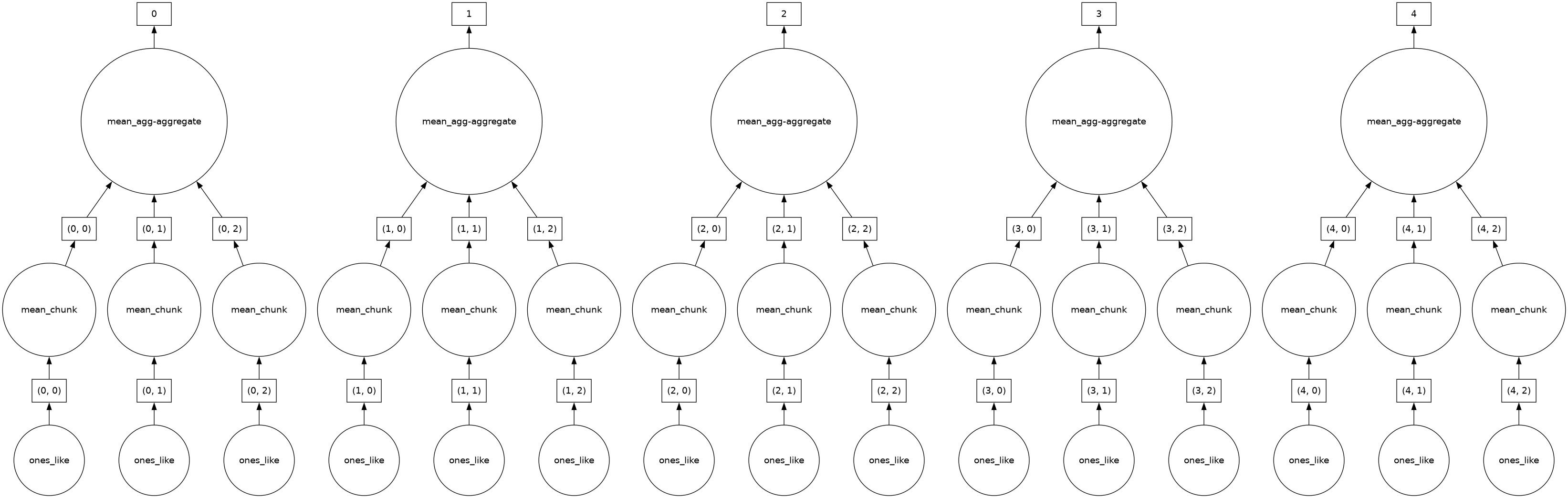
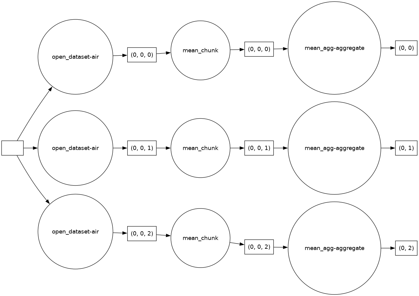
actual_range: [185.16 322.1 ]Dask actually constructs a graph of the required computation. Here it’s pretty simple: The full array is subdivided into 3 arrays. Dask will load each of these subarrays in a separate thread using the default single-machine scheduling. You can visualize dask ‘task graphs’ which represent the requested computation:
mean.data # dask array
|
||||||||||||||||
# visualize the graph for the underlying dask array
# we ask it to visualize the graph from left to right because it looks nicer
dask.visualize(mean.data, rankdir="LR")
Getting concrete values#
At some point, you will want to actually get concrete values (usually a numpy array) from dask.
There are two ways to compute values on dask arrays.
.compute()returns an xarray object just like a dask array.load()replaces the dask array in the xarray object with a numpy array. This is equivalent tods = ds.compute()
Tip
There is a third option : “persisting”. .persist() loads the values into distributed RAM. The values are computed but remain distributed across workers. So ds.air.persist() still returns a dask array. This is useful if you will be repeatedly using a dataset for computation but it is too large to load into local memory. You will see a persistent task on the dashboard. See the dask user guide for more on persisting
Exercise
Try running mean.compute and then examine mean after that. Is it still a dask array?
Solution
Computing returns a numpy array but does not modify in-place. So mean still contains a dask array.
Exercise
Now repeat that exercise with mean.load.
Solution
load modifies an Xarray object in-place so mean now contains a numpy array.
Distributed Clusters#
As your data volumes grow and algorithms get more complex it can be hard to print out task graph representations and understand what Dask is doing behind the scenes. Luckily, you can use Dask’s ‘Distributed’ scheduler to get very useful diagnotisic information.
First let’s set up a LocalCluster using dask.distributed.
You can use any kind of Dask cluster. This step is completely independent of xarray. While not strictly necessary, the dashboard provides a nice learning tool.
By default, Dask uses the current working directory for writing temporary files.
We choose to use a temporary scratch folder local_directory='/tmp' in the example below instead.
import os

# This piece of code is just for a correct dashboard link mybinder.org or other JupyterHub demos
import dask
from dask.distributed import Client

# if os.environ.get('JUPYTERHUB_USER'):
#    dask.config.set(**{"distributed.dashboard.link": "/user/{JUPYTERHUB_USER}/proxy/{port}/status"})

client = Client()
client
Client
Client-ee0cf9d9-7fb0-11f1-8c0e-7c1e52224af6
| Connection method: Cluster object | Cluster type: distributed.LocalCluster |
| Dashboard: http://127.0.0.1:8787/status |
Cluster Info
LocalCluster
b3d9d31a
| Dashboard: http://127.0.0.1:8787/status | Workers: 4 |
| Total threads: 4 | Total memory: 15.61 GiB |
| Status: running | Using processes: True |
Scheduler Info
Scheduler
Scheduler-195ba0fc-a584-4102-a417-0bfec4dbcf05
| Comm: tcp://127.0.0.1:33095 | Workers: 0 |
| Dashboard: http://127.0.0.1:8787/status | Total threads: 0 |
| Started: Just now | Total memory: 0 B |
Workers
Worker: 0
| Comm: tcp://127.0.0.1:46255 | Total threads: 1 |
| Dashboard: http://127.0.0.1:42387/status | Memory: 3.90 GiB |
| Nanny: tcp://127.0.0.1:36707 | |
| Local directory: /tmp/dask-scratch-space/worker-c5uttxdu | |
Worker: 1
| Comm: tcp://127.0.0.1:44263 | Total threads: 1 |
| Dashboard: http://127.0.0.1:32803/status | Memory: 3.90 GiB |
| Nanny: tcp://127.0.0.1:42123 | |
| Local directory: /tmp/dask-scratch-space/worker-kyjrjc83 | |
Worker: 2
| Comm: tcp://127.0.0.1:44955 | Total threads: 1 |
| Dashboard: http://127.0.0.1:39625/status | Memory: 3.90 GiB |
| Nanny: tcp://127.0.0.1:39769 | |
| Local directory: /tmp/dask-scratch-space/worker-ar5xyjxr | |
Worker: 3
| Comm: tcp://127.0.0.1:46647 | Total threads: 1 |
| Dashboard: http://127.0.0.1:43253/status | Memory: 3.90 GiB |
| Nanny: tcp://127.0.0.1:46603 | |
| Local directory: /tmp/dask-scratch-space/worker-upty6p6n | |
☝️ Click the Dashboard link above.
👈 Or click the “Search” 🔍 button in the dask-labextension dashboard.
Note
if using the dask-labextension, you should disable the ‘Simple’ JupyterLab interface (View -> Simple Interface), so that you can drag and rearrange whichever dashboards you want. The Workers and Task Stream are good to make sure the dashboard is working!
import dask.array

dask.array.ones((1000, 4), chunks=(2, 1)).compute()  # should see activity in dashboard
array([[1., 1., 1., 1.],
       [1., 1., 1., 1.],
       ...,
       [1., 1., 1., 1.],
       [1., 1., 1., 1.]], shape=(1000, 4))
Computation#
Let’s go back to our xarray DataSet, in addition to computing the mean, other operations such as indexing will automatically use whichever Dask Cluster we are connected to!
ds.air.isel(lon=1, lat=20)
<xarray.DataArray 'air' (time: 2920)> Size: 23kB
dask.array<chunksize=(2920,), meta=np.ndarray>
Coordinates:
  * time     (time) datetime64[ns] 23kB 2013-01-01 ... 2014-12-31T18:00:00
    lat      float32 4B 25.0
    lon      float32 4B 202.5
Attributes:
    long_name:     4xDaily Air temperature at sigma level 995
    units:         degK
    precision:     2
    GRIB_id:       11
    GRIB_name:     TMP
    var_desc:      Air temperature
    dataset:       NMC Reanalysis
    level_desc:    Surface
    statistic:     Individual Obs
    parent_stat:   Other
actual_range: [185.16 322.1 ]and more complicated operations…
rolling_mean = ds.air.rolling(time=5).mean()  # no activity on dashboard
rolling_mean  # contains dask array
<xarray.DataArray 'air' (time: 2920, lat: 25, lon: 53)> Size: 31MB
dask.array<chunksize=(2920, 9, 9), meta=np.ndarray>
Coordinates:
  * time     (time) datetime64[ns] 23kB 2013-01-01 ... 2014-12-31T18:00:00
  * lat      (lat) float32 100B 75.0 72.5 70.0 67.5 65.0 ... 22.5 20.0 17.5 15.0
  * lon      (lon) float32 212B 200.0 202.5 205.0 207.5 ... 325.0 327.5 330.0
Attributes:
    long_name:     4xDaily Air temperature at sigma level 995
    units:         degK
    precision:     2
    GRIB_id:       11
    GRIB_name:     TMP
    var_desc:      Air temperature
    dataset:       NMC Reanalysis
    level_desc:    Surface
    statistic:     Individual Obs
    parent_stat:   Other
actual_range: [185.16 322.1 ]timeseries = rolling_mean.isel(lon=1, lat=20) # no activity on dashboard
timeseries # contains dask array
<xarray.DataArray 'air' (time: 2920)> Size: 23kB
dask.array<chunksize=(2920,), meta=np.ndarray>
Coordinates:
  * time     (time) datetime64[ns] 23kB 2013-01-01 ... 2014-12-31T18:00:00
    lat      float32 4B 25.0
    lon      float32 4B 202.5
Attributes:
    long_name:     4xDaily Air temperature at sigma level 995
    units:         degK
    precision:     2
    GRIB_id:       11
    GRIB_name:     TMP
    var_desc:      Air temperature
    dataset:       NMC Reanalysis
    level_desc:    Surface
    statistic:     Individual Obs
    parent_stat:   Other
actual_range: [185.16 322.1 ]computed = rolling_mean.compute() # activity on dashboard
computed # has real numpy values
<xarray.DataArray 'air' (time: 2920, lat: 25, lon: 53)> Size: 31MB
nan nan nan nan nan nan nan nan ... 298.4 297.4 297.3 297.2 296.4 296.1 295.7
Coordinates:
  * time     (time) datetime64[ns] 23kB 2013-01-01 ... 2014-12-31T18:00:00
  * lat      (lat) float32 100B 75.0 72.5 70.0 67.5 65.0 ... 22.5 20.0 17.5 15.0
  * lon      (lon) float32 212B 200.0 202.5 205.0 207.5 ... 325.0 327.5 330.0
Attributes:
    long_name:     4xDaily Air temperature at sigma level 995
    units:         degK
    precision:     2
    GRIB_id:       11
    GRIB_name:     TMP
    var_desc:      Air temperature
    dataset:       NMC Reanalysis
    level_desc:    Surface
    statistic:     Individual Obs
    parent_stat:   Other
actual_range: [185.16 322.1 ]Note that mean still contains a dask array
rolling_mean
<xarray.DataArray 'air' (time: 2920, lat: 25, lon: 53)> Size: 31MB
dask.array<chunksize=(2920, 9, 9), meta=np.ndarray>
Coordinates:
  * time     (time) datetime64[ns] 23kB 2013-01-01 ... 2014-12-31T18:00:00
  * lat      (lat) float32 100B 75.0 72.5 70.0 67.5 65.0 ... 22.5 20.0 17.5 15.0
  * lon      (lon) float32 212B 200.0 202.5 205.0 207.5 ... 325.0 327.5 330.0
Attributes:
    long_name:     4xDaily Air temperature at sigma level 995
    units:         degK
    precision:     2
    GRIB_id:       11
    GRIB_name:     TMP
    var_desc:      Air temperature
    dataset:       NMC Reanalysis
    level_desc:    Surface
    statistic:     Individual Obs
    parent_stat:   Other
actual_range: [185.16 322.1 ]Tip
While these operations all work, not all of them are necessarily the optimal implementation for parallelism. Usually analysis pipelines need some tinkering and tweaking to get things to work. In particular read the user guidie recommendations for chunking.
Xarray data structures are first-class dask collections.#
This means you can do things like dask.compute(xarray_object),
dask.visualize(xarray_object), dask.persist(xarray_object). This works for
both DataArrays and Datasets
Exercise
Visualize the task graph for a few different computations on ds.air!
# Use this cell for the exercise
Finish up#
Gracefully shutdown our connection to the Dask cluster. This becomes more important when you are running on large HPC or Cloud servers rather than a laptop!
client.close()
Next#
See the Xarray user guide on dask.