Basic Computation#
In this lesson, we discuss how to do scientific computations with xarray objects. Our learning goals are as follows. By the end of the lesson, we will be able to:
Apply basic arithmetic and numpy functions to xarray DataArrays / Dataset.
Use Xarray’s label-aware reduction operations (e.g.
mean,sum) weighted reductions.Apply arbitrary functions to Xarray data via
apply_ufunc.Use Xarray’s broadcasting to compute on arrays of different dimensionality.
import matplotlib.pyplot as plt
import numpy as np
import xarray as xr

# Ask Xarray to not show data values by default
xr.set_options(display_expand_data=False)

%config InlineBackend.figure_format='retina'
Example Dataset#
First we load a dataset. We will use the NOAA Extended Reconstructed Sea Surface Temperature (ERSST) v5 product, a widely used and trusted gridded compilation of of historical data going back to 1854.
ds = xr.tutorial.load_dataset("ersstv5")
ds
<xarray.Dataset> Size: 40MB
Dimensions:    (time: 624, nbnds: 2, lat: 89, lon: 180)
Coordinates:
  * time       (time) datetime64[ns] 5kB 1970-01-01 1970-02-01 ... 2021-12-01
  * lat        (lat) float32 356B 88.0 86.0 84.0 82.0 ... -84.0 -86.0 -88.0
  * lon        (lon) float32 720B 0.0 2.0 4.0 6.0 ... 352.0 354.0 356.0 358.0
Dimensions without coordinates: nbnds
Data variables:
    time_bnds  (time, nbnds) float64 10kB 9.969e+36 9.969e+36 ... 9.969e+36
    sst        (time, lat, lon) float32 40MB -1.8 -1.8 -1.8 -1.8 ... nan nan nan
Attributes: (12/37)
    climatology:               Climatology is based on 1971-2000 SST, Xue, Y....
    description:               In situ data: ICOADS2.5 before 2007 and NCEP i...
    keywords_vocabulary:       NASA Global Change Master Directory (GCMD) Sci...
    keywords:                  Earth Science > Oceans > Ocean Temperature > S...
    instrument:                Conventional thermometers
    source_comment:            SSTs were observed by conventional thermometer...
    ...                        ...
    creator_url_original:      https://www.ncei.noaa.gov
    license:                   No constraints on data access or use
    comment:                   SSTs were observed by conventional thermometer...
    summary:                   ERSST.v5 is developed based on v4 after revisi...
    dataset_title:             NOAA Extended Reconstructed SST V5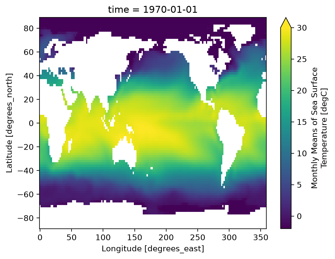
data_modified: 2022-06-07Let’s do some basic visualizations of the data, just to make sure it looks reasonable.
ds.sst.isel(time=0).plot(vmin=-2, vmax=30);
Arithmetic#
Xarray dataarrays and datasets work seamlessly with arithmetic operators and numpy array functions.
For example, imagine we want to convert the temperature (given in Celsius) to Kelvin:
sst_kelvin = ds.sst + 273.15
sst_kelvin
<xarray.DataArray 'sst' (time: 624, lat: 89, lon: 180)> Size: 40MB
271.4 271.4 271.4 271.4 271.4 271.4 271.4 271.4 ... nan nan nan nan nan nan nan
Coordinates:
  * time     (time) datetime64[ns] 5kB 1970-01-01 1970-02-01 ... 2021-12-01
  * lat      (lat) float32 356B 88.0 86.0 84.0 82.0 ... -82.0 -84.0 -86.0 -88.0
  * lon      (lon) float32 720B 0.0 2.0 4.0 6.0 8.0 ... 352.0 354.0 356.0 358.0
Attributes:
    long_name:     Monthly Means of Sea Surface Temperature
    units:         degC
    var_desc:      Sea Surface Temperature
    level_desc:    Surface
    statistic:     Mean
    dataset:       NOAA Extended Reconstructed SST V5
    parent_stat:   Individual Values
    actual_range:  [-1.8     42.32636]
valid_range: [-1.8 45. ]The dimensions and coordinates were preserved following the operation.
units attribute, which is used in plotting,
Xarray does not inherently understand units. However, xarray can integrate with pint, which provides full unit-aware operations. See pint-xarray for more.
Applying functions#
We can apply more complex functions to Xarray objects. Imagine we wanted to compute the following expression as a function of SST (\(\Theta\)) in Kelvin:
f = 0.5 * np.log(sst_kelvin**2)
f
<xarray.DataArray 'sst' (time: 624, lat: 89, lon: 180)> Size: 40MB
5.603 5.603 5.603 5.603 5.603 5.603 5.603 5.603 ... nan nan nan nan nan nan nan
Coordinates:
  * time     (time) datetime64[ns] 5kB 1970-01-01 1970-02-01 ... 2021-12-01
  * lat      (lat) float32 356B 88.0 86.0 84.0 82.0 ... -82.0 -84.0 -86.0 -88.0
  * lon      (lon) float32 720B 0.0 2.0 4.0 6.0 8.0 ... 352.0 354.0 356.0 358.0
Attributes:
    long_name:     Monthly Means of Sea Surface Temperature
    units:         degC
    var_desc:      Sea Surface Temperature
    level_desc:    Surface
    statistic:     Mean
    dataset:       NOAA Extended Reconstructed SST V5
    parent_stat:   Individual Values
    actual_range:  [-1.8     42.32636]
valid_range: [-1.8 45. ]Applying Arbitrary Functions#
It’s awesome that we can call np.log(ds) and have it “just work”. However, not
all third party libraries work this way.
numpy’s nan_to_num for example will return a numpy array
np.nan_to_num(ds.sst, nan=0)
array([[[-1.8, -1.8, -1.8, ..., -1.8, -1.8, -1.8],
        [-1.8, -1.8, -1.8, ..., -1.8, -1.8, -1.8],
        [-1.8, -1.8, -1.8, ..., -1.8, -1.8, -1.8],
        ...,
        [ 0. ,  0. ,  0. , ...,  0. ,  0. ,  0. ],
        [ 0. ,  0. ,  0. , ...,  0. ,  0. ,  0. ],
        [ 0. ,  0. ,  0. , ...,  0. ,  0. ,  0. ]],

       [[-1.8, -1.8, -1.8, ..., -1.8, -1.8, -1.8],
        [-1.8, -1.8, -1.8, ..., -1.8, -1.8, -1.8],
        [-1.8, -1.8, -1.8, ..., -1.8, -1.8, -1.8],
        ...,
        [ 0. ,  0. ,  0. , ...,  0. ,  0. ,  0. ],
        [ 0. ,  0. ,  0. , ...,  0. ,  0. ,  0. ],
        [ 0. ,  0. ,  0. , ...,  0. ,  0. ,  0. ]],

       ...,

       [[-1.8, -1.8, -1.8, ..., -1.8, -1.8, -1.8],
        [-1.8, -1.8, -1.8, ..., -1.8, -1.8, -1.8],
        [-1.8, -1.8, -1.8, ..., -1.8, -1.8, -1.8],
        ...,
        [ 0. ,  0. ,  0. , ...,  0. ,  0. ,  0. ],
        [ 0. ,  0. ,  0. , ...,  0. ,  0. ,  0. ],
        [ 0. ,  0. ,  0. , ...,  0. ,  0. ,  0. ]],

       [[-1.8, -1.8, -1.8, ..., -1.8, -1.8, -1.8],
        [-1.8, -1.8, -1.8, ..., -1.8, -1.8, -1.8],
        [-1.8, -1.8, -1.8, ..., -1.8, -1.8, -1.8],
        ...,
        [ 0. ,  0. ,  0. , ...,  0. ,  0. ,  0. ],
        [ 0. ,  0. ,  0. , ...,  0. ,  0. ,  0. ],
        [ 0. ,  0. ,  0. , ...,  0. ,  0. ,  0. ]]],
      shape=(624, 89, 180), dtype=float32)
It would be nice to keep our dimensions and coordinates.
We can accomplish this with xr.apply_ufunc
xr.apply_ufunc(np.nan_to_num, ds.sst, kwargs={"nan": 0})
<xarray.DataArray 'sst' (time: 624, lat: 89, lon: 180)> Size: 40MB
-1.8 -1.8 -1.8 -1.8 -1.8 -1.8 -1.8 -1.8 -1.8 ... 0.0 0.0 0.0 0.0 0.0 0.0 0.0 0.0
Coordinates:
  * time     (time) datetime64[ns] 5kB 1970-01-01 1970-02-01 ... 2021-12-01
  * lat      (lat) float32 356B 88.0 86.0 84.0 82.0 ... -82.0 -84.0 -86.0 -88.0
  * lon      (lon) float32 720B 0.0 2.0 4.0 6.0 8.0 ... 352.0 354.0 356.0 358.0
Attributes:
    long_name:     Monthly Means of Sea Surface Temperature
    units:         degC
    var_desc:      Sea Surface Temperature
    level_desc:    Surface
    statistic:     Mean
    dataset:       NOAA Extended Reconstructed SST V5
    parent_stat:   Individual Values
    actual_range:  [-1.8     42.32636]
valid_range: [-1.8 45. ]Tip
apply_ufunc is a powerful function. It has many options for doing more complicated things. Unfortunately, we don’t have time to go into more depth here. See the apply_ufunc tutorial material for more.
Reductions#
Reductions are functions that reduce the dimensionlity of our dataset. For example taking the mean sea surface temperature along time of our 3D data, we “reduce” the time dimension and are left with a 2D array.
Just like in numpy, we can reduce xarray DataArrays along any number of axes.
sst = ds.sst
sst.mean(axis=0)
<xarray.DataArray 'sst' (lat: 89, lon: 180)> Size: 64kB
-1.799 -1.799 -1.799 -1.799 -1.799 -1.8 -1.8 ... nan nan nan nan nan nan nan
Coordinates:
  * lat      (lat) float32 356B 88.0 86.0 84.0 82.0 ... -82.0 -84.0 -86.0 -88.0
  * lon      (lon) float32 720B 0.0 2.0 4.0 6.0 8.0 ... 352.0 354.0 356.0 358.0
Attributes:
    long_name:     Monthly Means of Sea Surface Temperature
    units:         degC
    var_desc:      Sea Surface Temperature
    level_desc:    Surface
    statistic:     Mean
    dataset:       NOAA Extended Reconstructed SST V5
    parent_stat:   Individual Values
    actual_range:  [-1.8     42.32636]
valid_range: [-1.8 45. ]However, rather than performing reductions by specifying axis (as in numpy), we can instead perform
them using dimension names. This turns out to be a huge convenience, particularly in
complex calculations it can be hard to remember which axis corresponds to
which dimension name:
sst.mean(dim="time")
<xarray.DataArray 'sst' (lat: 89, lon: 180)> Size: 64kB
-1.799 -1.799 -1.799 -1.799 -1.799 -1.8 -1.8 ... nan nan nan nan nan nan nan
Coordinates:
  * lat      (lat) float32 356B 88.0 86.0 84.0 82.0 ... -82.0 -84.0 -86.0 -88.0
  * lon      (lon) float32 720B 0.0 2.0 4.0 6.0 8.0 ... 352.0 354.0 356.0 358.0
Attributes:
    long_name:     Monthly Means of Sea Surface Temperature
    units:         degC
    var_desc:      Sea Surface Temperature
    level_desc:    Surface
    statistic:     Mean
    dataset:       NOAA Extended Reconstructed SST V5
    parent_stat:   Individual Values
    actual_range:  [-1.8     42.32636]
valid_range: [-1.8 45. ]You can reduce over multiple dimensions
sst.mean(["lat", "time"])
<xarray.DataArray 'sst' (lon: 180)> Size: 720B
11.8 11.61 11.83 11.86 11.64 11.58 10.6 ... 12.26 12.15 11.55 11.22 11.26 11.34
Coordinates:
  * lon      (lon) float32 720B 0.0 2.0 4.0 6.0 8.0 ... 352.0 354.0 356.0 358.0
Attributes:
    long_name:     Monthly Means of Sea Surface Temperature
    units:         degC
    var_desc:      Sea Surface Temperature
    level_desc:    Surface
    statistic:     Mean
    dataset:       NOAA Extended Reconstructed SST V5
    parent_stat:   Individual Values
    actual_range:  [-1.8     42.32636]
valid_range: [-1.8 45. ]If no dimension is specified, the reduction is applied across all dimensions.
sst.mean()
<xarray.DataArray 'sst' ()> Size: 4B
13.81
Attributes:
    long_name:     Monthly Means of Sea Surface Temperature
    units:         degC
    var_desc:      Sea Surface Temperature
    level_desc:    Surface
    statistic:     Mean
    dataset:       NOAA Extended Reconstructed SST V5
    parent_stat:   Individual Values
    actual_range:  [-1.8     42.32636]
valid_range: [-1.8 45. ]All of the standard numpy reductions (e.g. min, max, sum, std, etc.) are
available on both Datasets and DataArrays.
Exercise
Take the mean of sst in both longitude and latitude. Make a simple timeseries plot.
Solution
sst.mean(["lat", "lon"]).plot();