A Tour of Xarray Customizations

A Tour of Xarray Customizations#

Xarray is easily extensible. This means it is easy to add on to to build custom packages that tackle particular computational problems or supply domain specific functionality.

These packages can plug in to xarray in various different ways. They may build directly on top of xarray, or they may take advantage of some of xarray’s dedicated interfacing features:

Accessors (extensions)
Backend (filetype) entrypoint
Metadata attributes
Duck-array wrapping interface
Flexible indexes (coming soon!)

Here we introduce several popular or interesting extensions that are installable as their own packages (via conda and pip). These packages integrate with xarray using one or more of the features mentioned above.

hvplot, a powerful interactive plotting library
rioxarray, for working with geospatial raster data using rasterio
cf-xarray, for interpreting CF-compliant data
pint-xarray, for unit-aware computations using pint.

Specific examples for implementing your own xarray customizations using these interfacing features are available in the ADVANCED section of this book.

import xarray as xr
import numpy as np

Quick note on accessors#

Before we look at the packages we need to briefly introduce a feature they commonly use: “xarray accessors”.

The accessor-style syntax is used heavily by the other libraries we are about to cover.

For users, accessors just allow us to have a familiar dot (method-like) syntax on xarray objects, for example da.hvplot(), da.pint.quantify(), or da.cf.describe().

hvplot via accessors#

The HoloViews library makes great use of accessors to allow seamless plotting of xarray data using a completely different plotting backend (by default, xarray uses matplotlib).

We first need to import the code that registers the hvplot accessor

import hvplot.xarray

And now we can call the .hvplot method to plot using holoviews in the same way that we would have used .plot to plot using matplotlib.

ds = xr.tutorial.load_dataset("air_temperature")

ds['air'].isel(time=1).hvplot(cmap="fire")

For some more examples of how powerful HoloViews is see here.

Rioxarray via the backend entrypoint#

Rioxarray is a Python library that enhances Xarray’s ability to work with geospatial data and coordinate reference systems. Geographic information systems use GeoTIFF and many other formats to organize and store gridded, or raster, datasets.

The Geospatial Data Abstraction Library (GDAL) provides foundational drivers and geospatial algorithms, and the rasterio library provides a Pythonic interface to GDAL. Rioxarray brings key features of rasterio to Xarray:

A backend engine to read any format recognized by GDAL
A .rio accessor for rasterio’s geospatial algorithms such as reprojection

Below a couple brief examples to illustrate these features:

import rioxarray  # ensure you have rioxarray installed in your environment

You can explicitly use rioxarray’s ‘rasterio’ engine to load myriad geospatial raster formats. Below is a Cloud-Optimized Geotiff from an AWS public dataset of synthetic aperture radar data over Washington, State, USA. overview_level=4 is an argument specific to the rasterio engine that allows opening a pre-computed lower resolution “overview” of the data.

The spatial_ref coordinate is added by rioxarray to store standardized geospatial Coordinate Reference System (CRS) information. We can access that information and additional methods via the .rio accessor:

da.rio.crs

CRS.from_epsg(32610)

EPSG refers to ‘European Petroleum Survey Group’, a database of the many CRS definitions for our Planet used over the years! EPSG=32610 is the “UTM 10N” CRS, with coordinate units in meters. Let’s say you want longitude,latitude coordinate points in degrees instead. You’d have to reproject this data:

Note that that the size of the data has changed as well as the coordinate values. This is typical of reprojection, as your data must be resampled and often interpolated to match the new CRS grid! A quick plot will compare the results of our reprojected data:

import panel as pn

img1 = da.sel(band=1).hvplot.image(
    x='x', y='y', rasterize=True, cmap='gray', clim=(0, 0.5), title='UTM'
)
img2 = da_lonlat.sel(band=1).hvplot.image(
    rasterize=True, cmap='gray', clim=(0, 0.5), title='LON/LAT'
)

pn.Column(img1, img2)

Pint via duck array wrapping#

Why use pint#

Pint defines physical units, allowing you to work with numpy-like arrays which track the units of your values through computations.

Pint defines a numpy-like array class called pint.Quantity, which is made up of a numpy array and a pint.Unit instance.

from pint import Unit

# you can create a pint.Quantity by multiplying a value by a pint.Unit
d = np.array(10) * Unit("metres")
d

10 meter

These units are automatically propagated through operations

t = 1 * Unit("seconds")
v = d / t
v

10.0 meter/second

Or if the operation involves inconsistent units, a pint.DimensionalityError is raised.

d + t

---------------------------------------------------------------------------
DimensionalityError                       Traceback (most recent call last)
Cell In[17], line 1
----> 1 d + t

File ~/micromamba/envs/xarray-tutorial/lib/python3.11/site-packages/pint/facets/plain/quantity.py:841, in PlainQuantity.__add__(self, other)
    838 if isinstance(other, datetime.datetime):
    839     return self.to_timedelta() + other
--> 841 return self._add_sub(other, operator.add)

File ~/micromamba/envs/xarray-tutorial/lib/python3.11/site-packages/pint/facets/plain/quantity.py:103, in check_implemented.<locals>.wrapped(self, *args, **kwargs)
    101 elif isinstance(other, list) and other and isinstance(other[0], type(self)):
    102     return NotImplemented
--> 103 return f(self, *args, **kwargs)

File ~/micromamba/envs/xarray-tutorial/lib/python3.11/site-packages/pint/facets/plain/quantity.py:743, in PlainQuantity._add_sub(self, other, op)
    740     return self.__class__(magnitude, units)
    742 if not self.dimensionality == other.dimensionality:
--> 743     raise DimensionalityError(
    744         self._units, other._units, self.dimensionality, other.dimensionality
    745     )
    747 # Next we define some variables to make if-clauses more readable.
    748 self_non_mul_units = self._get_non_multiplicative_units()

DimensionalityError: Cannot convert from 'meter' ([length]) to 'second' ([time])

pint inside xarray objects#

We have already seen that xarray can wrap numpy arrays or dask arrays, but in fact xarray can wrap any type of array that behaves similarly to a numpy array. Using this feature we can store a pint.Quantity array inside an xarray DataArray

da = xr.DataArray(d)
da

<xarray.DataArray ()>
<Quantity(10, 'meter')>

We can see that the data type stored within the DataArray is a Quantity object, rather than just a np.ndarray object, and the units of the data are displayed in the repr.

The reason this works is that a pint.Quantity array is what we call a “duck array”, in that it behaves so similarly to a numpy.ndarray that xarray can treat them the same way. (See python duck typing)

pint-xarray#

The convenience package pint-xarray makes it easier to get the benefits of pint whilst working with xarray objects.

It provides utility accessor methods for promoting xarray data to pint quantities (which we call “quantifying”) in various ways and for manipulating the resulting objects.

# to be able to read unit attributes following the CF conventions
import cf_xarray.units
import pint_xarray

xr.set_options(display_expand_data=False)

<xarray.core.options.set_options at 0x7f62c40ac450>

pint-xarray provides the .pint accessor, which firstly allows us to easily extract the units of our data

da.pint.units

meter

The .pint.quantify() accessor gives us various ways to convert normal xarray data to be unit-aware.

Note

It is preferred to use .pint.quantify() to convert xarray data to use pint rather than explicitly creating a pint.Quantity array and placing it inside the xarray object, because pint-xarray will handle various subtleties involving dask etc.

We can explicitly specify the units we want

da = xr.DataArray([4.5, 6.7, 3.8], dims="time")
da.pint.quantify("V")

<xarray.DataArray (time: 3)>
[V] 4.5 6.7 3.8
Dimensions without coordinates: time

Or if the data has a “units” entry in its .attrs metadata dictionary, we can automatically use that to convert each variable.

For example, the xarray tutorial dataset we opened earlier has units in its attributes

ds.air.attrs['units']

'degK'

which we can automatically read with .pint.quantify():

quantified_air = ds.pint.quantify()
quantified_air

<xarray.Dataset>
Dimensions:  (time: 2920, lat: 25, lon: 53)
Coordinates:
  * lat      (lat) float32 75.0 72.5 70.0 67.5 65.0 ... 25.0 22.5 20.0 17.5 15.0
  * lon      (lon) float32 200.0 202.5 205.0 207.5 ... 322.5 325.0 327.5 330.0
  * time     (time) datetime64[ns] 2013-01-01 ... 2014-12-31T18:00:00
Data variables:
    air      (time, lat, lon) float32 [K] 241.2 242.5 243.5 ... 296.19 295.69
Attributes:
    Conventions:  COARDS
    title:        4x daily NMC reanalysis (1948)
    description:  Data is from NMC initialized reanalysis\n(4x/day).  These a...
    platform:     Model
    references:   http://www.esrl.noaa.gov/psd/data/gridded/data.ncep.reanaly...

Here we have actually gone even further, and used cf-xarray to automatically interpret cf-compliant units in the .attrs to valid pint units. This automatically happened just as a result of importing cf-xarray above.

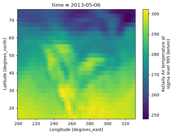
When we plot quantified data with xarray the correct units will automatically appear on the plot

quantified_air["air"].isel(time=500).plot();

../_images/dc67faa0e006e75eebe28c21b8ccb11448f4d0fd6326b29a08b956b7d06af77c.png

If we want to cast the pint arrays back to numpy arrays, we can use .pint.dequantify(), which will also write the current units back out to the .attrs["units"] field

Exercise 22

Write a function which will raise a pint.DimensionalityError if supplied with Xarray DataArray with the wrong units.

Solution to Exercise 22

from pint import DimensionalityError


def special_science_function(distance):
    if distance.pint.units != "miles":
        raise DimensionalityError(
            "this function will only give the correct answer if the input is in units of miles"
        )

Exercise 23

Try this on some of your data!

After you have imported pint-xarray (and maybe cf-xarray) as above, start with something like

ds = xr.open_dataset(my_data).pint.quantify()

Take a look at the pint-xarray documentation or the pint documentation if you get stuck.

The wider world…#

There are many other libraries in the wider xarray ecosystem. For a list of a few packages we particularly like for geoscience work see here, and for a more exhaustive list see here.

Magnitude	[4.5 6.7 3.8]
Units	volt