Computational Patterns#
Often when writing code we repeat certain patterns, whether we realize it or not. If you have learned to write list comprehensions, you are taking advantage of a “control pattern”. Often, these patterns are so common that many packages have built in functions to implement them.
Quoting the toolz documentation:
The Toolz library contains dozens of patterns like map and groupby. Learning a core set (maybe a dozen) covers the vast majority of common programming tasks often done by hand. A rich vocabulary of core control functions conveys the following benefits:
You identify new patterns
You make fewer errors in rote coding
You can depend on well tested and benchmarked implementations
The same is true for xarray.
See also
The concepts covered here, particularly the emphasis on deleting for loops and focusing on large elements of the computation, are very related to the array programming style or paradigm. See this SciPy 2023 tutorial on “Thinking Like Arrays” by Jim Pivarski if you are interested in these ideas.
Motivation / Learning goals#
Learn what high-level computational patterns are available in Xarray.
Learn that these patterns replace common uses of the
forloop.Identify when you are re-implementing an existing computational pattern.
Implement that pattern using built-in Xarray functionality.
Understand the difference between
mapandreduce.
Xarray’s high-level patterns#
Xarray allows you to leverage dataset metadata to write more readable analysis code. The metadata is stored with the data; not in your head.
Dimension names:
dim="latitude"instead ofaxis=0Coordinate “labels”: or axis tick labels.
data.sel(latitude=45)instead ofdata[10]
Xarray also provides computational patterns that cover many data analysis tasks.
Xarray provides methods for high-level analysis patterns:
rolling: Operate on rolling or sliding (fixed length, overlapping) windows of your data e.g. running mean.coarsen: Operate on blocks (fixed length) of your data (downsample).groupby: Parse data into groups (using an exact value) and operate on each one (reduce data).groupby_bins: GroupBy after discretizing a numeric (non-exact, e.g. float) variable.resample: [Groupby specialized for time axes. Either downsample or upsample your data.]weighted: Weight your data before reducing.
Note
The documentation links in this tutorial point to the DataArray implementations of each function, but they are also available for DataSet objects.
Load example dataset#
import numpy as np
import xarray as xr
import matplotlib.pyplot as plt
# reduce figure size
plt.rcParams["figure.dpi"] = 90
xr.set_options(keep_attrs=True, display_expand_data=False)
da = xr.tutorial.load_dataset("air_temperature", engine="netcdf4").air
monthly = da.resample(time="ME").mean()
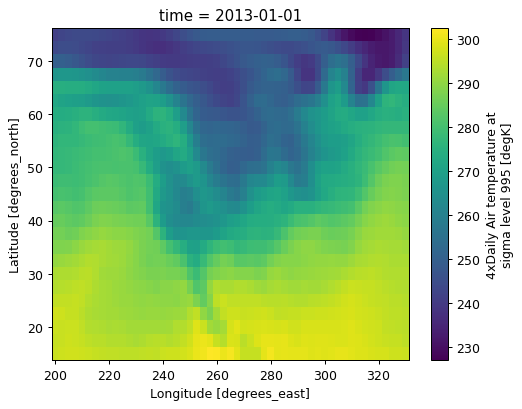
data = da.isel(time=0)
data.plot();
da
<xarray.DataArray 'air' (time: 2920, lat: 25, lon: 53)> Size: 31MB
241.2 242.5 243.5 244.0 244.1 243.9 ... 297.9 297.4 297.2 296.5 296.2 295.7
Coordinates:
  * lat      (lat) float32 100B 75.0 72.5 70.0 67.5 65.0 ... 22.5 20.0 17.5 15.0
  * lon      (lon) float32 212B 200.0 202.5 205.0 207.5 ... 325.0 327.5 330.0
  * time     (time) datetime64[ns] 23kB 2013-01-01 ... 2014-12-31T18:00:00
Attributes:
    long_name:     4xDaily Air temperature at sigma level 995
    units:         degK
    precision:     2
    GRIB_id:       11
    GRIB_name:     TMP
    var_desc:      Air temperature
    dataset:       NMC Reanalysis
    level_desc:    Surface
    statistic:     Individual Obs
    parent_stat:   Other
actual_range: [185.16 322.1 ]Identifying high-level computation patterns#
or, when should I use these functions?
Consider a common use case. We want to complete some “task” for each of “something”. The “task” might be a computation (e.g. mean, median, plot). The “something” could be a group of array values (e.g. pixels) or segments of time (e.g. monthly or seasonally).
Often, our solution to this type of problem is to write a for loop. Say we want the average air temperature for each month across the entire domain (all lat and lon values):
months = [1, 2, 3, 4, 5, 6, 7, 8, 9, 10, 11, 12]
avg_temps = []

# for loop
for mon in months:
    # filter data, split out in to groups
    subset = da[da["time.month"] == mon]
    # do some computation
    avg = subset.mean()
    # append to existing results
    avg_temps.append(avg.item())

print(avg_temps)
[273.4167740722314, 273.13103153669846, 275.1137128427892, 278.5469922646425, 283.2990779677319, 287.56573034648716, 289.9069213031189, 290.08913216739444, 287.4137458496152, 283.6811443399555, 277.96778471723593, 274.35104421814054]
This pattern is the GroupBy pattern.
An easy conceptual next step for this example (but still using our for loop) would be to use Xarray’s groupby function to create an iterator that does the work of grouping our data by month and looping over each month.
[273.4167740722314, 273.13103153669846, 275.1137128427892, 278.5469922646425, 283.2990779677319, 287.56573034648716, 289.9069213031189, 290.08913216739444, 287.4137458496152, 283.6811443399555, 277.96778471723593, 274.35104421814054]
Writing a for-loop here is not wrong, but it can quickly become cumbersome if you have a complex function to apply and it will take a while to compute on a large dataset (you may even run out of memory). Parallelizing the computation would take a lot of additional work.
Xarray’s functionality instead allows us to do the same computation in one line of code (plus, the computation is optimized and ready to take advantage of parallel compute resources)!
# note the use of the ellipses here
# for easy comparison to the for loop above
avg_temps = da.groupby("time.month").mean(...)
print(avg_temps.data)
[273.41677407 273.13103154 275.11371284 278.54699226 283.29907797
 287.56573035 289.9069213  290.08913217 287.41374585 283.68114434
 277.96778472 274.35104422]
Note
By default, da.mean() (and df.mean()) will calculate the mean by reducing your data over all dimensions (unless you specify otherwise using the dim kwarg). The default behavior of .mean() on a groupby is to calculate the mean over all dimensions of the variable you are grouping by - but not all the dimensions of the object you are operating on. To compute the mean across all dimensions of a groupby, we must specify ... for all dimensions (or use the dim kwarg to specify which dimensions to reduce by).
Here we showed an example for computing a mean over a certain period of time (months), which ultimately uses the GroupBy function to group together observations with similar characteristics that are scattered through the dataset. The transition from loops to a built-in function is similar for rolling and coarsen over sequential windows of values (e.g. pixels) instead of “groups” of time.
Read on through this tutorial to learn some of the incredible ways to use Xarray to avoid writing long for-loops and efficiently complete computational analyses on your data.
See also
For a more complex example (identifying flood events - including their start and end date - from rainfall data) illustrating the transition from for loops to high level computation tools, see this discussion. The original 40 lines of code, including nested for loops, was streamlined into a ~15 line workflow without any loops.
Concept refresher: “index space” vs “label space”#
data
<xarray.DataArray 'air' (lat: 25, lon: 53)> Size: 11kB
241.2 242.5 243.5 244.0 244.1 243.9 ... 298.0 297.8 297.6 296.9 296.8 296.6
Coordinates:
  * lat      (lat) float32 100B 75.0 72.5 70.0 67.5 65.0 ... 22.5 20.0 17.5 15.0
  * lon      (lon) float32 212B 200.0 202.5 205.0 207.5 ... 325.0 327.5 330.0
    time     datetime64[ns] 8B 2013-01-01
Attributes:
    long_name:     4xDaily Air temperature at sigma level 995
    units:         degK
    precision:     2
    GRIB_id:       11
    GRIB_name:     TMP
    var_desc:      Air temperature
    dataset:       NMC Reanalysis
    level_desc:    Surface
    statistic:     Individual Obs
    parent_stat:   Other
actual_range: [185.16 322.1 ]# index space
data[10, :] # 10th element along the first axis; ¯\_(ツ)_/¯
<xarray.DataArray 'air' (lon: 53)> Size: 424B
277.3 277.4 277.8 278.6 279.5 280.1 ... 280.5 282.9 284.7 286.1 286.9 286.6
Coordinates:
    lat      float32 4B 50.0
  * lon      (lon) float32 212B 200.0 202.5 205.0 207.5 ... 325.0 327.5 330.0
    time     datetime64[ns] 8B 2013-01-01
Attributes:
    long_name:     4xDaily Air temperature at sigma level 995
    units:         degK
    precision:     2
    GRIB_id:       11
    GRIB_name:     TMP
    var_desc:      Air temperature
    dataset:       NMC Reanalysis
    level_desc:    Surface
    statistic:     Individual Obs
    parent_stat:   Other
actual_range: [185.16 322.1 ]# slightly better index space
data.isel(lat=10) # slightly better, 10th element in latitude
<xarray.DataArray 'air' (lon: 53)> Size: 424B
277.3 277.4 277.8 278.6 279.5 280.1 ... 280.5 282.9 284.7 286.1 286.9 286.6
Coordinates:
    lat      float32 4B 50.0
  * lon      (lon) float32 212B 200.0 202.5 205.0 207.5 ... 325.0 327.5 330.0
    time     datetime64[ns] 8B 2013-01-01
Attributes:
    long_name:     4xDaily Air temperature at sigma level 995
    units:         degK
    precision:     2
    GRIB_id:       11
    GRIB_name:     TMP
    var_desc:      Air temperature
    dataset:       NMC Reanalysis
    level_desc:    Surface
    statistic:     Individual Obs
    parent_stat:   Other
actual_range: [185.16 322.1 ]# "label" space
data.sel(lat=50) # much better! lat=50°N
<xarray.DataArray 'air' (lon: 53)> Size: 424B
277.3 277.4 277.8 278.6 279.5 280.1 ... 280.5 282.9 284.7 286.1 286.9 286.6
Coordinates:
    lat      float32 4B 50.0
  * lon      (lon) float32 212B 200.0 202.5 205.0 207.5 ... 325.0 327.5 330.0
    time     datetime64[ns] 8B 2013-01-01
Attributes:
    long_name:     4xDaily Air temperature at sigma level 995
    units:         degK
    precision:     2
    GRIB_id:       11
    GRIB_name:     TMP
    var_desc:      Air temperature
    dataset:       NMC Reanalysis
    level_desc:    Surface
    statistic:     Individual Obs
    parent_stat:   Other
actual_range: [185.16 322.1 ]# What I wanted to do
data.sel(lat=50)
# What I had to do (if I wasn't using xarray)
data[10, :]
<xarray.DataArray 'air' (lon: 53)> Size: 424B
277.3 277.4 277.8 278.6 279.5 280.1 ... 280.5 282.9 284.7 286.1 286.9 286.6
Coordinates:
    lat      float32 4B 50.0
  * lon      (lon) float32 212B 200.0 202.5 205.0 207.5 ... 325.0 327.5 330.0
    time     datetime64[ns] 8B 2013-01-01
Attributes:
    long_name:     4xDaily Air temperature at sigma level 995
    units:         degK
    precision:     2
    GRIB_id:       11
    GRIB_name:     TMP
    var_desc:      Air temperature
    dataset:       NMC Reanalysis
    level_desc:    Surface
    statistic:     Individual Obs
    parent_stat:   Other
actual_range: [185.16 322.1 ]Xarray provides patterns in both “index space” and “label space”#
Index space#
These are sequential windowed operations with a window of a fixed size.
Label space#
These are windowed operations with irregular windows based on your data. Members of a single group may be non-sequential and scattered through the dataset.
groupby: Parse data into groups (using an exact value) and operate on each one (reduce data).groupby_bins: GroupBy after discretizing a numeric (non-exact, e.g. float) variable.resample: Groupby specialized for time axes. Either downsample or upsample your data.
add some “loop” versions to show what a user might come up with that could be turned into one of these pattern operations
Index space: windows of fixed width#
Sliding windows of fixed length: rolling#
Supports common reductions :
sum,mean,count,std,varetc.Returns object of same shape as input
Pads with NaNs to make this happen
Supports multiple dimensions
Here’s the dataset
data.plot();
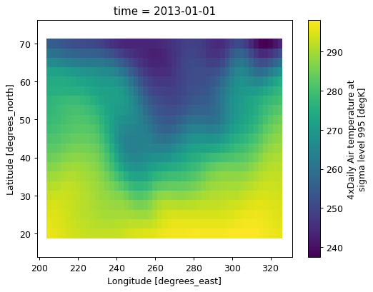
And now smoothed 5 point running mean in lat and lon
data.rolling(lat=5, lon=5, center=True).mean().plot();
Apply an existing numpy-only function with reduce#
In some cases, we may want to apply a sliding window function using rolling that is not built in to Xarray. In these cases we can still leverage the sliding windows of rolling and apply our own function with reduce.
The reduce method on Xarray objects (e.g. DataArray, Dataset) expects a function that can receive and return plain arrays (e.g. numpy), as in each of the “windows” provided by the rolling iterator. This is in contrast to the map method on DataArray and Dataset objects, which expects a function that can receive and return Xarray objects.
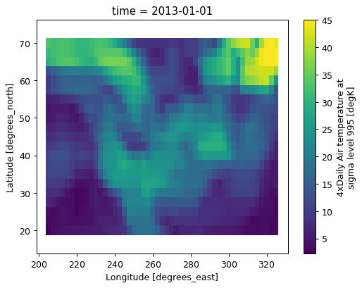
Here’s an example function: np.ptp.
data.rolling(lat=5, lon=5, center=True).reduce(np.ptp).plot();
Exercise
Calculate the rolling mean in 5 point bins along both latitude and longitude using
rolling(...).reduce
Solution
# exactly equivalent to data.rolling(...).mean()
data.rolling(lat=5, lon=5, center=True).reduce(np.mean).plot();
View the rolling operation as a Xarray object with construct#
In the above examples, we plotted the outputs of our rolling operations. Xarray makes it easy to integrate the outputs from rolling directly into the DataArray using the xarray.computation.rolling.DataArrayRolling.construct method.
simple = xr.DataArray(np.arange(10), dims="time", coords={"time": np.arange(10)})
simple
<xarray.DataArray (time: 10)> Size: 80B
0 1 2 3 4 5 6 7 8 9
Coordinates:
  * time     (time) int64 80B 0 1 2 3 4 5 6 7 8 9
# adds a new dimension "window"
simple.rolling(time=5, center=True).construct("window")
<xarray.DataArray (time: 10, window: 5)> Size: 400B
nan nan 0.0 1.0 2.0 nan 0.0 1.0 2.0 3.0 ... 7.0 8.0 9.0 nan 7.0 8.0 9.0 nan nan
Coordinates:
  * time     (time) int64 80B 0 1 2 3 4 5 6 7 8 9
Dimensions without coordinates: window
Note
Because .construct() only returns a “view” (not a copy) of the original data object (i.e. it is not operating “in-place”), in order to “save” the results you would need to rewrite the original object: simple = simple.rolling(time=5, center=True).construct("window").
Exercise
Calculate the 5 point running mean in time using rolling.construct
Solution
simple.rolling(time=5, center=True).construct("window").mean("window")
construct is clever.
It constructs a view of the original array, so it is memory-efficient.
It does something sensible for dask arrays (though generally you want big chunksizes for the dimension you’re sliding along).
It also works with rolling along multiple dimensions!
Advanced: Another construct example#
This is a 2D rolling example; we need to provide two new dimension names.
data.rolling(lat=5, lon=5, center=True).construct(lat="lat_roll", lon="lon_roll")
<xarray.DataArray 'air' (lat: 25, lon: 53, lat_roll: 5, lon_roll: 5)> Size: 265kB
nan nan nan nan nan nan nan nan nan nan ... nan nan nan nan nan nan nan nan nan
Coordinates:
  * lat      (lat) float32 100B 75.0 72.5 70.0 67.5 65.0 ... 22.5 20.0 17.5 15.0
  * lon      (lon) float32 212B 200.0 202.5 205.0 207.5 ... 325.0 327.5 330.0
    time     datetime64[ns] 8B 2013-01-01
Dimensions without coordinates: lat_roll, lon_roll
Attributes:
    long_name:     4xDaily Air temperature at sigma level 995
    units:         degK
    precision:     2
    GRIB_id:       11
    GRIB_name:     TMP
    var_desc:      Air temperature
    dataset:       NMC Reanalysis
    level_desc:    Surface
    statistic:     Individual Obs
    parent_stat:   Other
actual_range: [185.16 322.1 ]Block windows of fixed length: coarsen#
For non-overlapping windows or “blocks” use coarsen. The syntax is very similar to rolling. You will need to specify how you want Xarray to handle the boundary if the length of the dimension is not a multiple of the block size.
Supports common reductions :
sum,mean,count,std,varetc.Does not return an object of same shape as input
Allows controls over behaviour at boundaries
Supports multiple dimensions
data
<xarray.DataArray 'air' (lat: 25, lon: 53)> Size: 11kB
241.2 242.5 243.5 244.0 244.1 243.9 ... 298.0 297.8 297.6 296.9 296.8 296.6
Coordinates:
  * lat      (lat) float32 100B 75.0 72.5 70.0 67.5 65.0 ... 22.5 20.0 17.5 15.0
  * lon      (lon) float32 212B 200.0 202.5 205.0 207.5 ... 325.0 327.5 330.0
    time     datetime64[ns] 8B 2013-01-01
Attributes:
    long_name:     4xDaily Air temperature at sigma level 995
    units:         degK
    precision:     2
    GRIB_id:       11
    GRIB_name:     TMP
    var_desc:      Air temperature
    dataset:       NMC Reanalysis
    level_desc:    Surface
    statistic:     Individual Obs
    parent_stat:   Other
actual_range: [185.16 322.1 ]data.plot();
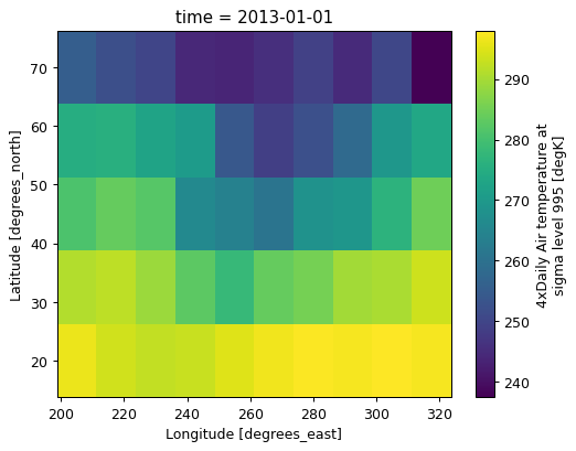
data.coarsen(lat=5, lon=5, boundary="trim").mean()
<xarray.DataArray 'air' (lat: 5, lon: 10)> Size: 400B
255.3 252.1 249.8 244.3 243.8 245.7 ... 295.0 296.8 297.6 297.2 298.0 297.1
Coordinates:
  * lat      (lat) float32 20B 70.0 57.5 45.0 32.5 20.0
  * lon      (lon) float32 40B 205.0 217.5 230.0 242.5 ... 292.5 305.0 317.5
    time     datetime64[ns] 8B 2013-01-01
Attributes:
    long_name:     4xDaily Air temperature at sigma level 995
    units:         degK
    precision:     2
    GRIB_id:       11
    GRIB_name:     TMP
    var_desc:      Air temperature
    dataset:       NMC Reanalysis
    level_desc:    Surface
    statistic:     Individual Obs
    parent_stat:   Other
actual_range: [185.16 322.1 ](data.coarsen(lat=5, lon=5, boundary="trim").mean().plot())
<matplotlib.collections.QuadMesh at 0x7f305d107290>
Coarsen supports reduce for custom reductions#
Exercise
Use coarsen.reduce to apply np.ptp in 5x5 (lat x lon) point blocks to data
Solution
data.coarsen(lat=5, lon=5, boundary="trim").reduce(np.ptp).plot();
Coarsen supports construct for block reshaping and storing outputs#
Tip
coarsen.construct is usually a good alternative to np.reshape
A simple example splits a 2-year long monthly 1D time series into a 2D array shaped (year x month)
<xarray.DataArray (time: 24)> Size: 192B
1 2 3 4 5 6 7 8 9 10 11 12 1 2 3 4 5 6 7 8 9 10 11 12
Coordinates:
  * time     (time) int64 192B 1 2 3 4 5 6 7 8 9 ... 16 17 18 19 20 21 22 23 24
# break "time" into two new dimensions: "year", "month"
months.coarsen(time=12).construct(time=("year", "month"))
<xarray.DataArray (year: 2, month: 12)> Size: 192B
1 2 3 4 5 6 7 8 9 10 11 12 1 2 3 4 5 6 7 8 9 10 11 12
Coordinates:
    time     (year, month) int64 192B 1 2 3 4 5 6 7 8 ... 18 19 20 21 22 23 24
Dimensions without coordinates: year, monthNote two things:
The
timedimension was also reshaped.The new dimensions
yearandmonthdon’t have any coordinate labels associated with them.
What if the data had say 23 instead of 24 values (months.isel(time=slice(1, None))? In that case we specify a different boundary (the default boundary="exact" worked above); here we pad to 24 values.
months.isel(time=slice(1, None)).coarsen(time=12, boundary="pad").construct(time=("year", "month"))
<xarray.DataArray (year: 2, month: 12)> Size: 192B
2.0 3.0 4.0 5.0 6.0 7.0 8.0 9.0 10.0 ... 5.0 6.0 7.0 8.0 9.0 10.0 11.0 12.0 nan
Coordinates:
    time     (year, month) float64 192B 2.0 3.0 4.0 5.0 ... 22.0 23.0 24.0 nan
Dimensions without coordinates: year, monthThis adds values at the end of the array (see the ‘nan’ at the end of the time coordinate?), which is not so sensible for this
problem. We have some control of the padding through the side kwarg to coarsen. For side="right" we get more sensible output.
months.isel(time=slice(1, None)).coarsen(time=12, boundary="pad", side="right").construct(
    time=("year", "month")
)
<xarray.DataArray (year: 2, month: 12)> Size: 192B
nan 2.0 3.0 4.0 5.0 6.0 7.0 8.0 9.0 ... 4.0 5.0 6.0 7.0 8.0 9.0 10.0 11.0 12.0
Coordinates:
    time     (year, month) float64 192B nan 2.0 3.0 4.0 ... 21.0 22.0 23.0 24.0
Dimensions without coordinates: year, monthNote that coarsen pads with NaNs. For more control over padding, use
DataArray.pad explicitly.
(
    months.isel(time=slice(1, None))
    .pad(time=(1, 0), constant_values=-1)
    .coarsen(time=12)
    .construct(time=("year", "month"))
)
<xarray.DataArray (year: 2, month: 12)> Size: 192B
-1 2 3 4 5 6 7 8 9 10 11 12 1 2 3 4 5 6 7 8 9 10 11 12
Coordinates:
    time     (year, month) float64 192B nan 2.0 3.0 4.0 ... 21.0 22.0 23.0 24.0
Dimensions without coordinates: year, monthNote
The value specified in .pad only applies the fill_value to the array, not to coordinate variables.
This is why the first value of time in the above example is NaN and not -1.
Exercise
Reshape the time dimension of the DataArray monthly to year x
month and visualize the seasonal cycle for two years at 250°E
Solution
# splits time dimension into year x month
year_month = monthly.coarsen(time=12).construct(time=("year", "month"))

# assign a nice coordinate value for month
year_month["month"] = [
    "jan",
    "feb",
    "mar",
    "apr",
    "may",
    "jun",
    "jul",
    "aug",
    "sep",
    "oct",
    "nov",
    "dec",
]

# assign a nice coordinate value for year
year_month["year"] = [2013, 2014]

# seasonal cycle for two years
year_month.sel(lon=250).plot.contourf(col="year", x="month", y="lat")
Exercise
Calculate the rolling 4 month average, averaged across years. (This exercise came up during a live lecture).
Solution
We first reshape using
coarsen.constructto addyearas a new dimension.Apply
rollingon the month dimension.It turns out that
roll.mean(["year", "month"])doesn’t work. So we useroll.constructto get a DataArray with a new dimensionwindowand then take the mean overwindowandyear
reshaped = months.coarsen(time=12).construct(time=("year", "month"))
roll = reshaped.rolling(month=4, center=True)
roll.construct("window").mean(["window", "year"])
Summary#
Delete your for loops. Use rolling and coarsen for fixed size windowing operations.
rollingfor overlapping windowscoarsenfor non-overlapping windows.
Both provide the usual reductions as methods (.mean() and friends), and also
reduce and construct for custom operations.
Label space “windows” or bins : GroupBy#
Sometimes the windows you want are not regularly spaced or even defined by a grid.
For instance, grouping data by month (which have varying numbers of days) or the results of an image classification.
The GroupBy functions are essentially a generalization of coarsen:
groupby: divide data into distinct groups, e.g. climatologies, composites. Works best when the “group identifiers” or “labels” are exact and can be determined using equality (==), e.g. characters or integers. Remember that floats are not exact values.groupby_bins: Use binning operations, e.g. histograms, to group your data.resample: Specialized implementation of GroupBy specifically for time grouping (so far), allows you to change sampling frequency of dataset.
Note
Both groupby_bins and resample are implemented as groupby with a specific way of constructing group labels. The GroupBy pattern is very flexible!
Deconstructing GroupBy#
The GroupBy workflow is commonly called “split-apply-combine”.
Split : break dataset into groups
Apply : apply an operation, for instance a reduction like
meanCombine : concatenate results from apply step along a new “group” dimension
illustrated in this neat schematic from Project Pythia:
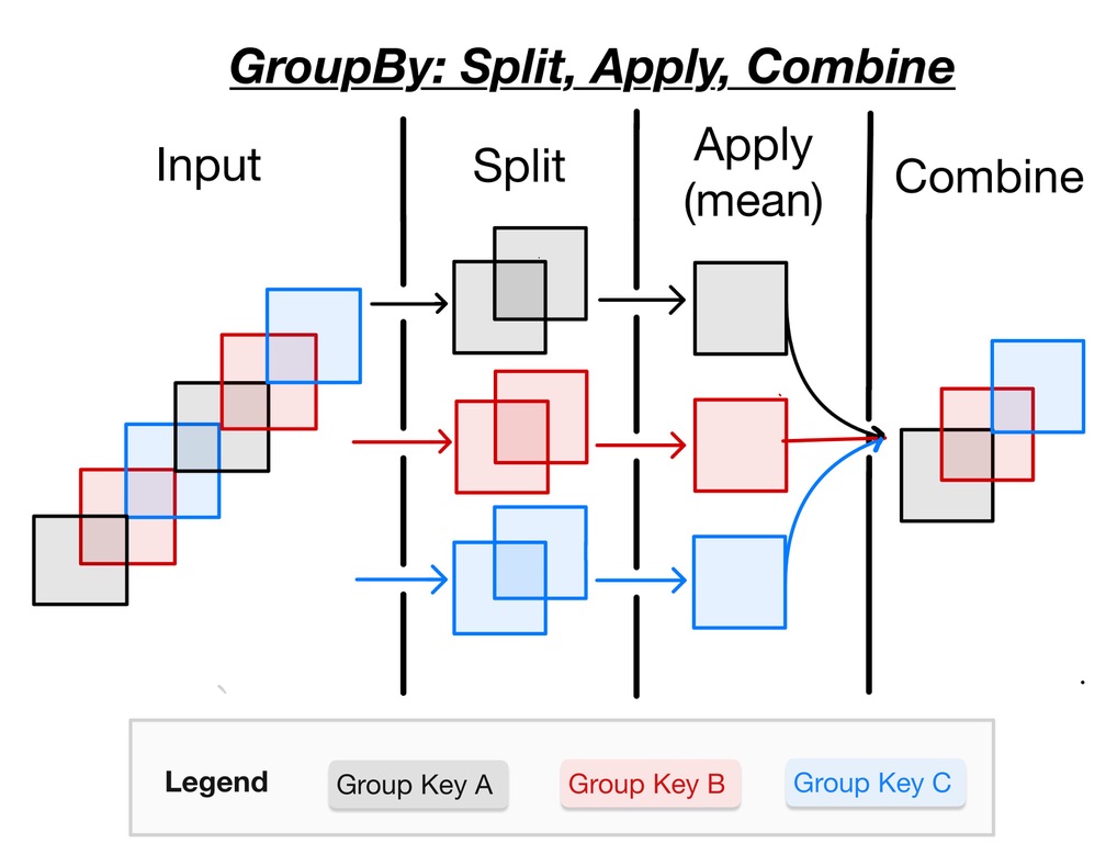
But really there is a “hidden” first step: identifying groups (also called “factorization” or sometimes “binning”). Usually this is the hard part.
In reality the workflow is: “identify groups” → “split into groups” → “apply function” → “combine results”.
# recall our earlier DataArray
da
<xarray.DataArray 'air' (time: 2920, lat: 25, lon: 53)> Size: 31MB
241.2 242.5 243.5 244.0 244.1 243.9 ... 297.9 297.4 297.2 296.5 296.2 295.7
Coordinates:
  * lat      (lat) float32 100B 75.0 72.5 70.0 67.5 65.0 ... 22.5 20.0 17.5 15.0
  * lon      (lon) float32 212B 200.0 202.5 205.0 207.5 ... 325.0 327.5 330.0
  * time     (time) datetime64[ns] 23kB 2013-01-01 ... 2014-12-31T18:00:00
Attributes:
    long_name:     4xDaily Air temperature at sigma level 995
    units:         degK
    precision:     2
    GRIB_id:       11
    GRIB_name:     TMP
    var_desc:      Air temperature
    dataset:       NMC Reanalysis
    level_desc:    Surface
    statistic:     Individual Obs
    parent_stat:   Other
actual_range: [185.16 322.1 ]# GroupBy returns an iterator that traverses the specified groups, here by month.
# Notice that groupby is clever enough for us to leave out the `.dt` before `.month`
# we would need to specify to access the month data directly, as in `da.time.dt.month`.
da.groupby("time.month")
<DataArrayGroupBy, grouped over 1 grouper(s), 12 groups in total:
    'month': UniqueGrouper('month'), 12/12 groups with labels 1, 2, 3, 4, 5, 6, 7, 8, 9, 10, 11, 12>
# for each group (e.g. the air temperature in a given month for all the years),
# compute the mean
da.groupby("time.month").mean()
<xarray.DataArray 'air' (month: 12, lat: 25, lon: 53)> Size: 127kB
246.3 246.4 246.2 245.8 245.2 244.6 ... 298.1 298.0 298.0 297.6 297.6 297.5
Coordinates:
  * lat      (lat) float32 100B 75.0 72.5 70.0 67.5 65.0 ... 22.5 20.0 17.5 15.0
  * lon      (lon) float32 212B 200.0 202.5 205.0 207.5 ... 325.0 327.5 330.0
  * month    (month) int64 96B 1 2 3 4 5 6 7 8 9 10 11 12
Attributes:
    long_name:     4xDaily Air temperature at sigma level 995
    units:         degK
    precision:     2
    GRIB_id:       11
    GRIB_name:     TMP
    var_desc:      Air temperature
    dataset:       NMC Reanalysis
    level_desc:    Surface
    statistic:     Individual Obs
    parent_stat:   Other
actual_range: [185.16 322.1 ]Notice that since we have averaged over all the years for each month, our resulting DataArray no longer has a “year” coordinate.
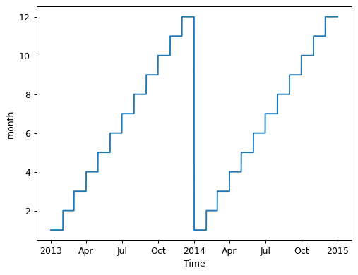
If we want to see how Xarray identifies “groups” for the monthly climatology computation, we can plot our input to groupby. GroupBy is clever enough to figure out how many values there are an thus how many groups to make.
da["time.month"].plot();
Similarly for binning (remember this is useful when the parameter you are binning over is not “exact”, like a float),
data.groupby_bins("lat", bins=[20, 35, 40, 45, 50])
<DataArrayGroupBy, grouped over 1 grouper(s), 4 groups in total:
    'lat_bins': BinGrouper('lat'), 4/4 groups with labels (20,, 35], (35,, 40], ..., (45,, 50]>
and resampling…
da.resample(time="ME")
<DataArrayResample, grouped over 1 grouper(s), 24 groups in total:
    '__resample_dim__': TimeResampler('__resample_dim__'), 24/24 groups with labels 2013-01-31, ..., 2014-12-31>
Note
Resampling is changing the frequency of our data to monthly (for two years), so we have 24 bins. GroupBy is taking the average across all data in the same month for two years, so we have 12 bins.
Constructing group labels#
If the automatic group detection doesn’t work for your problem then these functions are useful for constructing specific “group labels” in many cases
numpy.digitize for binning
numpy.searchsorted supports many other data types
pandas.factorize supports characters, strings etc.
pandas.cut for binning
“Datetime components” of Xarray DataArrays
Do you know of any more? (Send in a pull request to update this list!)
Tip
Xarray uses pandas.factorize for groupby and pandas.cut for groupby_bins.
“Datetime components” for creating groups#
See a full list here
These can be accessed in a few different ways as illustrated below.
da.time
<xarray.DataArray 'time' (time: 2920)> Size: 23kB
2013-01-01 2013-01-01T06:00:00 ... 2014-12-31T12:00:00 2014-12-31T18:00:00
Coordinates:
  * time     (time) datetime64[ns] 23kB 2013-01-01 ... 2014-12-31T18:00:00
Attributes:
    standard_name:  time
long_name: Timeda.time.dt.day
<xarray.DataArray 'day' (time: 2920)> Size: 23kB
1 1 1 1 2 2 2 2 3 3 3 3 4 4 4 4 ... 28 28 28 29 29 29 29 30 30 30 30 31 31 31 31
Coordinates:
  * time     (time) datetime64[ns] 23kB 2013-01-01 ... 2014-12-31T18:00:00
Attributes:
    standard_name:  time
long_name: Timeda["time.day"]
<xarray.DataArray 'day' (time: 2920)> Size: 23kB
1 1 1 1 2 2 2 2 3 3 3 3 4 4 4 4 ... 28 28 28 29 29 29 29 30 30 30 30 31 31 31 31
Coordinates:
  * time     (time) datetime64[ns] 23kB 2013-01-01 ... 2014-12-31T18:00:00
da.time.dt.season
<xarray.DataArray 'season' (time: 2920)> Size: 35kB
'DJF' 'DJF' 'DJF' 'DJF' 'DJF' 'DJF' ... 'DJF' 'DJF' 'DJF' 'DJF' 'DJF' 'DJF'
Coordinates:
  * time     (time) datetime64[ns] 23kB 2013-01-01 ... 2014-12-31T18:00:00
Attributes:
    standard_name:  time
long_name: TimeConstruct and use custom labels#
Custom seasons with numpy.isin.#
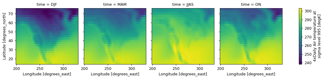
We want to group over four seasons: DJF, MAM, JJAS, ON - this makes physical sense in the Indian Ocean basin.
Start by extracting months.
month = da.time.dt.month.data
month
array([ 1, 1, 1, ..., 12, 12, 12], shape=(2920,))
Create a new empty array
myseason = np.full(month.shape, "    ")
myseason
array(['    ', '    ', '    ', ..., '    ', '    ', '    '],
      shape=(2920,), dtype='<U4')
Use isin to assign custom seasons,
Turn our new seasonal group array into a DataArray.
myseason_da = da.time.copy(data=myseason)
myseason_da
<xarray.DataArray 'time' (time: 2920)> Size: 47kB
'DJF' 'DJF' 'DJF' 'DJF' 'DJF' 'DJF' ... 'DJF' 'DJF' 'DJF' 'DJF' 'DJF' 'DJF'
Coordinates:
  * time     (time) datetime64[ns] 23kB 2013-01-01 ... 2014-12-31T18:00:00
Attributes:
    standard_name:  time
long_name: Time(
# Calculate climatology
da.groupby(myseason_da)
.mean()
# reindex to get seasons in logical order (not alphabetical order)
.reindex(time=["DJF", "MAM", "JJAS", "ON"])
.plot(col="time")
)
<xarray.plot.facetgrid.FacetGrid at 0x7f305d269820>
floor, ceil and round on time#
Additional functionality in the datetime accessor allows us to effectively “resample” our time data to remove roundoff errors in timestamps.
da.time
<xarray.DataArray 'time' (time: 2920)> Size: 23kB
2013-01-01 2013-01-01T06:00:00 ... 2014-12-31T12:00:00 2014-12-31T18:00:00
Coordinates:
  * time     (time) datetime64[ns] 23kB 2013-01-01 ... 2014-12-31T18:00:00
Attributes:
    standard_name:  time
long_name: Time# remove roundoff error in timestamps
# floor to daily frequency
da.time.dt.floor("D")
<xarray.DataArray 'floor' (time: 2920)> Size: 23kB
2013-01-01 2013-01-01 2013-01-01 2013-01-01 ... 2014-12-31 2014-12-31 2014-12-31
Coordinates:
  * time     (time) datetime64[ns] 23kB 2013-01-01 ... 2014-12-31T18:00:00
Attributes:
    standard_name:  time
long_name: Timestrftime is another powerful option#
So useful and so unintuitive that it has its own website: https://strftime.org/
This is useful to avoid merging “Feb-29” and “Mar-01” for a daily climatology
da.time.dt.strftime("%b-%d")
<xarray.DataArray 'strftime' (time: 2920)> Size: 23kB
'Jan-01' 'Jan-01' 'Jan-01' 'Jan-01' ... 'Dec-31' 'Dec-31' 'Dec-31' 'Dec-31'
Coordinates:
  * time     (time) datetime64[ns] 23kB 2013-01-01 ... 2014-12-31T18:00:00
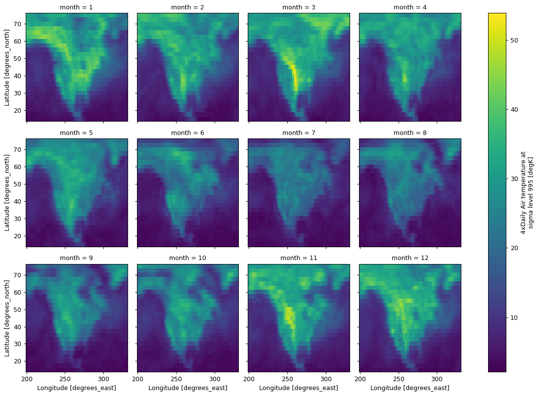
Custom reductions with GroupBy.reduce#
Analogous to rolling, reduce and map apply custom reductions to groupby_bins and resample.
(da.groupby("time.month").reduce(np.ptp).plot(col="month", col_wrap=4))
<xarray.plot.facetgrid.FacetGrid at 0x7f305d1470e0>
Tip
map is for functions that expect and return xarray objects (see also Dataset.map). reduce is for functions that expect and return plain arrays (like Numpy or SciPy functions).
Viewing the GroupBy operation on your DataArray or DataSet#
GroupBy does not provide a construct method, because all the groups need not be the same “length” (e.g. months can have 28, 29, 30, or 31 days).
Instead looping over groupby objects is possible#
Because groupby returns an iterator that loops over each group, it is easy to loop over groupby objects. You can also iterate over rolling and coarsen objects, however this approach is usually quite slow.
Maybe you want to plot data in each group separately:
for label, group in da.groupby("time.month"):
    print(label)
1
2
3
4
5
6
7
8
9
10
11
12
group is a DataArray containing data for all December days (because the last printed label value is 12, so the last group value is for December).
group
<xarray.DataArray 'air' (time: 248, lat: 25, lon: 53)> Size: 3MB
268.8 266.6 263.8 260.7 257.6 254.8 ... 297.9 297.4 297.2 296.5 296.2 295.7
Coordinates:
  * lat      (lat) float32 100B 75.0 72.5 70.0 67.5 65.0 ... 22.5 20.0 17.5 15.0
  * lon      (lon) float32 212B 200.0 202.5 205.0 207.5 ... 325.0 327.5 330.0
  * time     (time) datetime64[ns] 2kB 2013-12-01 ... 2014-12-31T18:00:00
Attributes:
    long_name:     4xDaily Air temperature at sigma level 995
    units:         degK
    precision:     2
    GRIB_id:       11
    GRIB_name:     TMP
    var_desc:      Air temperature
    dataset:       NMC Reanalysis
    level_desc:    Surface
    statistic:     Individual Obs
    parent_stat:   Other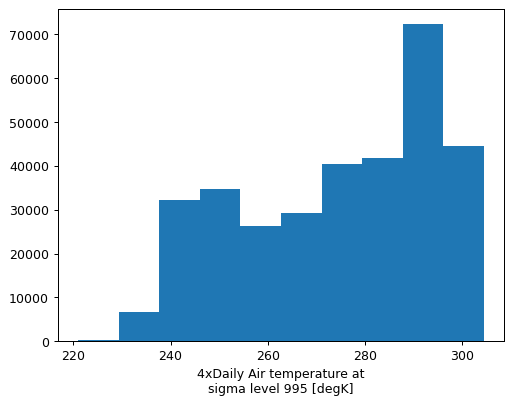
actual_range: [185.16 322.1 ]Maybe you want a histogram of December temperatures?
group.plot.hist()
(array([  218.,  6763., 32167., 34735., 26251., 29243., 40491., 41906.,
        72286., 44540.]),
 array([221.   , 229.339, 237.678, 246.017, 254.356, 262.695, 271.034,
        279.373, 287.712, 296.051, 304.39 ]),
 <BarContainer object of 10 artists>)
Remember, this example is just to show how you could operate on each group object in a groupby operation. If we wanted to just explore the December (or March) data, we should just filter for it directly:
da[da["time.month"] == 12].plot.hist()
(array([  218.,  6763., 32167., 34735., 26251., 29243., 40491., 41906.,
        72286., 44540.]),
 array([221.   , 229.339, 237.678, 246.017, 254.356, 262.695, 271.034,
        279.373, 287.712, 296.051, 304.39 ]),
 <BarContainer object of 10 artists>)
In most cases, avoid a for loop using map#
map enables us to apply functions that expect xarray Datasets or DataArrays. This makes it easy to perform calculations on the grouped data, add the results from each group back to the original object, and avoid having to manually combine results (using concat).
Tip
The implementation of map is a for loop. We like map because it’s cleaner.
def iqr(gb_da, dim):
    """Calculates interquartile range"""
    return (gb_da.quantile(q=0.75, dim=dim) - gb_da.quantile(q=0.25, dim=dim)).rename("iqr")


da.groupby("time.month").map(iqr, dim="time")
<xarray.DataArray 'iqr' (month: 12, lat: 25, lon: 53)> Size: 127kB
7.528 7.425 7.025 6.65 6.153 6.135 6.127 ... 0.9 0.9 0.855 1.0 1.3 1.432 1.5
Coordinates:
  * lat      (lat) float32 100B 75.0 72.5 70.0 67.5 65.0 ... 22.5 20.0 17.5 15.0
  * lon      (lon) float32 212B 200.0 202.5 205.0 207.5 ... 325.0 327.5 330.0
  * month    (month) int64 96B 1 2 3 4 5 6 7 8 9 10 11 12
Attributes:
    long_name:     4xDaily Air temperature at sigma level 995
    units:         degK
    precision:     2
    GRIB_id:       11
    GRIB_name:     TMP
    var_desc:      Air temperature
    dataset:       NMC Reanalysis
    level_desc:    Surface
    statistic:     Individual Obs
    parent_stat:   Other
actual_range: [185.16 322.1 ]Summary#
Xarray provides methods for high-level analysis patterns:
rolling: Operate on rolling or sliding (fixed length, overlapping) windows of your data e.g. running mean.coarsen: Operate on blocks (fixed length) of your data (downsample).groupby: Parse data into groups (using an exact value) and operate on each one (reduce data).groupby_bins: GroupBy after discretizing a numeric (non-exact, e.g. float) variable.resample: [Groupby specialized for time axes. Either downsample or upsample your data.]weighted: Weight your data before reducing.
Xarray also provides a consistent interface to make using those patterns easy:
Iterate over the operators (
rolling,coarsen,groupby,groupby_bins,resample).Apply functions that accept numpy-like arrays with
reduce.Reshape to a new xarray object with
.construct(rolling,coarsenonly).Apply functions that accept xarray objects with
map(groupby,groupby_bins,resampleonly).