Indexing and Selecting Data#
Learning Objectives#
Understanding the difference between position and label-based indexing
Select data by position using
.iselwith values or slicesSelect data by label using
.selwith values or slicesUse nearest-neighbor lookups with
.selSelect timeseries data by date/time with values or slices
Introduction#
Xarray offers extremely flexible indexing routines that combine the best features of NumPy and Pandas for data selection.
The most basic way to access elements of a DataArray object is to use Python’s [] syntax, such as array[i, j], where i and j are both integers.
As xarray objects can store coordinates corresponding to each dimension of an array, label-based indexing is also possible (e.g. .sel(latitude=0), similar to pandas.DataFrame.loc). In label-based indexing, the element position i is automatically looked-up from the coordinate values.
By leveraging the labeled dimensions and coordinates provided by Xarray, users can effortlessly access, subset, and manipulate data along multiple axes, enabling complex operations such as slicing, masking, and aggregating data based on specific criteria.
This indexing and selection capability of Xarray not only enhances data exploration and analysis workflows but also promotes reproducibility and efficiency by providing a convenient interface for working with multi-dimensional data structures.
Quick Overview#
In total, xarray supports four different kinds of indexing, as described below and summarized in this table:
Dimension lookup |
Index lookup |
|
|
|---|---|---|---|
Positional |
By integer |
|
not available |
Positional |
By label |
|
not available |
By name |
By integer |
|
|
By name |
By label |
|
|
In this tutorial, first we cover the positional indexing and label-based indexing, next we will cover more advanced techniques such as nearest neighbor lookups.
First, let’s import packages:
import xarray as xr

xr.set_options(display_expand_attrs=False, display_expand_data=False);
Here we’ll use air temperature tutorial dataset from the National Center for Environmental Prediction.
ds = xr.tutorial.load_dataset("air_temperature")
ds
<xarray.Dataset> Size: 31MB
Dimensions:  (lat: 25, time: 2920, lon: 53)
Coordinates:
  * lat      (lat) float32 100B 75.0 72.5 70.0 67.5 65.0 ... 22.5 20.0 17.5 15.0
  * lon      (lon) float32 212B 200.0 202.5 205.0 207.5 ... 325.0 327.5 330.0
  * time     (time) datetime64[ns] 23kB 2013-01-01 ... 2014-12-31T18:00:00
Data variables:
    air      (time, lat, lon) float64 31MB 241.2 242.5 243.5 ... 296.2 295.7
Attributes: (5)da = ds["air"]
Position-based Indexing#
Indexing a DataArray directly works (mostly) just like it does for numpy ndarrays, except that the returned object is always another DataArray:
NumPy Positional Indexing#
When working with numpy, indexing is done by position (slices/ranges/scalars).
For example:
np_array = ds["air"].data  # numpy array
np_array.shape
(2920, 25, 53)
Indexing is 0-based in NumPy:
np_array[1, 0, 0]
np.float64(242.1)
Similarly, we can select a range in NumPy:
# extract a time-series for one spatial location
np_array[:, 20, 40]
array([295. , 294.4 , 294.5 , ..., 297.29, 297.79, 297.99], shape=(2920,))
Positional Indexing with Xarray#
Xarray offers extremely flexible indexing routines that combine the best features of NumPy and pandas for data selection.
NumPy style indexing with Xarray#
NumPy style indexing works exactly the same with Xarray but it also preserves labels and metadata.
This approach however does not take advantage of the dimension names and coordinate location information that is present in a Xarray object.
da[:, 20, 40]
<xarray.DataArray 'air' (time: 2920)> Size: 23kB
295.0 294.4 294.5 295.4 295.2 294.4 ... 297.2 297.7 297.3 297.3 297.8 298.0
Coordinates:
    lat      float32 4B 25.0
    lon      float32 4B 300.0
  * time     (time) datetime64[ns] 23kB 2013-01-01 ... 2014-12-31T18:00:00
Attributes: (11)Positional Indexing Using Dimension Names#
Remembering the axis order can be challenging even with 2D arrays:
is
np_array[0,3]the first row and third column or first column and third row?or did I store these samples by row or by column when I saved the data?!.
The difficulty is compounded with added dimensions.
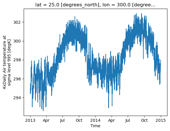
Xarray objects eliminate much of the mental overhead by allowing indexing using dimension names instead of axes numbers:
da.isel(lat=20, lon=40).plot();
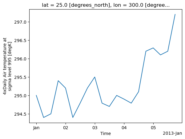
Slicing is also possible similarly:
da.isel(time=slice(0, 20), lat=20, lon=40).plot();
Note
Using the isel method, the user can choose/slice the specific elements from a Dataset or DataArray.
Indexing a DataArray directly works (mostly) just like it does for numpy arrays, except that the returned object is always another DataArray; however,when indexing with multiple arrays, positional indexing in Xarray behaves differently compared to NumPy.
Caution
Positional indexing deviates from the NumPy behavior when indexing with multiple arrays.
We can show this with an example:
np_array[:, [0, 1], [0, 1]].shape
(2920, 2)
da[:, [0, 1], [0, 1]].shape
(2920, 2, 2)
Please note how the dimension of the DataArray() object is different from the numpy.ndarray.
Tip
However, users can still achieve NumPy-like pointwise indexing across multiple labeled dimensions by using Xarray vectorized indexing techniques. We will delve further into this topic in the advanced indexing notebook.
So far, we have explored positional indexing, which relies on knowing the exact indices. But, what if you wanted to select data specifically for a particular latitude? It becomes challenging to determine the corresponding indices in such cases. Xarray reduce this complexity by introducing label-based indexing.
Label-based Indexing#
To select data by coordinate labels instead of integer indices we can use the same syntax, using sel instead of isel:
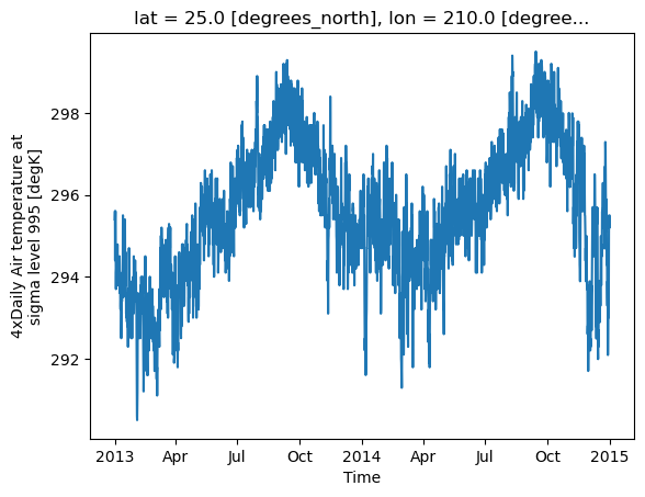
For example, let’s select all data for Lat 25 °N and Lon 210 °E using sel :
da.sel(lat=25, lon=210).plot();
Show code cell output
Similarly we can do slicing or filter a range using the .slice function:
# demonstrate slicing
da.sel(lon=slice(210, 215))
<xarray.DataArray 'air' (time: 2920, lat: 25, lon: 3)> Size: 2MB
244.1 243.9 243.6 243.4 242.4 241.7 ... 298.2 298.1 297.8 298.9 298.7 298.4
Coordinates:
  * lat      (lat) float32 100B 75.0 72.5 70.0 67.5 65.0 ... 22.5 20.0 17.5 15.0
  * lon      (lon) float32 12B 210.0 212.5 215.0
  * time     (time) datetime64[ns] 23kB 2013-01-01 ... 2014-12-31T18:00:00
Attributes: (11)
<xarray.DataArray 'air' (time: 2920, lat: 11, lon: 3)> Size: 771kB
279.5 280.1 280.6 279.4 280.3 281.3 ... 295.0 294.6 294.2 295.5 295.6 295.1
Coordinates:
  * lat      (lat) float32 44B 50.0 47.5 45.0 42.5 40.0 ... 32.5 30.0 27.5 25.0
  * lon      (lon) float32 12B 210.0 212.5 215.0
  * time     (time) datetime64[ns] 23kB 2013-01-01 ... 2014-12-31T18:00:00
Attributes: (11)
Dropping using drop_sel#
If instead of selecting data we want to drop it, we can use drop_sel method with syntax similar to sel:
da.drop_sel(lat=50.0, lon=200.0)
<xarray.DataArray 'air' (time: 2920, lat: 24, lon: 52)> Size: 29MB
242.5 243.5 244.0 244.1 243.9 243.6 ... 297.9 297.4 297.2 296.5 296.2 295.7
Coordinates:
  * lat      (lat) float32 96B 75.0 72.5 70.0 67.5 65.0 ... 22.5 20.0 17.5 15.0
  * lon      (lon) float32 208B 202.5 205.0 207.5 210.0 ... 325.0 327.5 330.0
  * time     (time) datetime64[ns] 23kB 2013-01-01 ... 2014-12-31T18:00:00
Attributes: (11)
So far, all the above will require us to specify exact coordinate values, but what if we don’t have the exact values? We can use nearest neighbor lookups to address this issue:
Nearest Neighbor Lookups#
The label based selection methods sel() support method and tolerance keyword argument. The method parameter allows for enabling nearest neighbor (inexact) lookups by use of the methods pad, backfill or nearest:
da.sel(lat=52.25, lon=251.8998, method="nearest")
<xarray.DataArray 'air' (time: 2920)> Size: 23kB
262.7 263.2 270.9 274.1 273.3 270.6 ... 247.3 253.4 261.6 264.2 265.2 267.0
Coordinates:
    lat      float32 4B 52.5
    lon      float32 4B 252.5
  * time     (time) datetime64[ns] 23kB 2013-01-01 ... 2014-12-31T18:00:00
Attributes: (11)tolerance argument limits the maximum distance for valid matches with an inexact lookup:
da.sel(lat=52.25, lon=251.8998, method="nearest", tolerance=2)
<xarray.DataArray 'air' (time: 2920)> Size: 23kB
262.7 263.2 270.9 274.1 273.3 270.6 ... 247.3 253.4 261.6 264.2 265.2 267.0
Coordinates:
    lat      float32 4B 52.5
    lon      float32 4B 252.5
  * time     (time) datetime64[ns] 23kB 2013-01-01 ... 2014-12-31T18:00:00
Attributes: (11)Tip
All of these indexing methods work on the dataset too!
We can also use these methods to index all variables in a dataset simultaneously, returning a new dataset:
ds.sel(lat=52.25, lon=251.8998, method="nearest")
<xarray.Dataset> Size: 47kB
Dimensions:  (time: 2920)
Coordinates:
    lat      float32 4B 52.5
    lon      float32 4B 252.5
  * time     (time) datetime64[ns] 23kB 2013-01-01 ... 2014-12-31T18:00:00
Data variables:
    air      (time) float64 23kB 262.7 263.2 270.9 274.1 ... 264.2 265.2 267.0
Attributes: (5)Datetime Indexing#
Datetime indexing is a critical feature when working with time series data, which is a common occurrence in many fields, including finance, economics, and environmental sciences. Essentially, datetime indexing allows you to select data points or a series of data points that correspond to certain date or time criteria. This becomes essential for time-series analysis where the date or time information associated with each data point can be as critical as the data point itself.
Let’s see some of the techniques to perform datetime indexing in Xarray:
Selecting data based on single datetime#
Let’s say we have a Dataset ds and we want to select data at a particular date and time, for instance, ‘2013-01-01’ at 6AM. We can do this by using the sel (select) method, like so:
ds.sel(time="2013-01-01 06:00")
<xarray.Dataset> Size: 11kB
Dimensions:  (lat: 25, lon: 53)
Coordinates:
  * lat      (lat) float32 100B 75.0 72.5 70.0 67.5 65.0 ... 22.5 20.0 17.5 15.0
  * lon      (lon) float32 212B 200.0 202.5 205.0 207.5 ... 325.0 327.5 330.0
    time     datetime64[ns] 8B 2013-01-01T06:00:00
Data variables:
    air      (lat, lon) float64 11kB 242.1 242.7 243.1 ... 296.4 296.4 296.6
Attributes: (5)By default, datetime selection will return a range of values that match the provided string. For e.g. time="2013-01-01" will return all timestamps for that day (4 of them here):
ds.sel(time="2013-01-01")
<xarray.Dataset> Size: 43kB
Dimensions:  (lat: 25, time: 4, lon: 53)
Coordinates:
  * lat      (lat) float32 100B 75.0 72.5 70.0 67.5 65.0 ... 22.5 20.0 17.5 15.0
  * lon      (lon) float32 212B 200.0 202.5 205.0 207.5 ... 325.0 327.5 330.0
  * time     (time) datetime64[ns] 32B 2013-01-01 ... 2013-01-01T18:00:00
Data variables:
    air      (time, lat, lon) float64 42kB 241.2 242.5 243.5 ... 298.0 297.9
Attributes: (5)We can use this feature to select all points in a year:
ds.sel(time="2014")
<xarray.Dataset> Size: 15MB
Dimensions:  (lat: 25, time: 1460, lon: 53)
Coordinates:
  * lat      (lat) float32 100B 75.0 72.5 70.0 67.5 65.0 ... 22.5 20.0 17.5 15.0
  * lon      (lon) float32 212B 200.0 202.5 205.0 207.5 ... 325.0 327.5 330.0
  * time     (time) datetime64[ns] 12kB 2014-01-01 ... 2014-12-31T18:00:00
Data variables:
    air      (time, lat, lon) float64 15MB 252.3 251.2 250.0 ... 296.2 295.7
Attributes: (5)or a month:
ds.sel(time="2014-May")
<xarray.Dataset> Size: 1MB
Dimensions:  (lat: 25, time: 124, lon: 53)
Coordinates:
  * lat      (lat) float32 100B 75.0 72.5 70.0 67.5 65.0 ... 22.5 20.0 17.5 15.0
  * lon      (lon) float32 212B 200.0 202.5 205.0 207.5 ... 325.0 327.5 330.0
  * time     (time) datetime64[ns] 992B 2014-05-01 ... 2014-05-31T18:00:00
Data variables:
    air      (time, lat, lon) float64 1MB 264.9 265.0 265.0 ... 296.2 296.2
Attributes: (5)Selecting data for a range of dates#
Now, let’s say we want to select data between a certain range of dates. We can still use the sel method, but this time we will combine it with slice:
# This will return a subset of the dataset corresponding to the entire year of 2013.
ds.sel(time=slice("2013-01-01", "2013-12-31"))
<xarray.Dataset> Size: 15MB
Dimensions:  (lat: 25, time: 1460, lon: 53)
Coordinates:
  * lat      (lat) float32 100B 75.0 72.5 70.0 67.5 65.0 ... 22.5 20.0 17.5 15.0
  * lon      (lon) float32 212B 200.0 202.5 205.0 207.5 ... 325.0 327.5 330.0
  * time     (time) datetime64[ns] 12kB 2013-01-01 ... 2013-12-31T18:00:00
Data variables:
    air      (time, lat, lon) float64 15MB 241.2 242.5 243.5 ... 295.1 294.7
Attributes: (5)Note
The slice function takes two arguments, start and stop, to make a slice that includes these endpoints. When we use slice with the sel method, it provides an efficient way to select a range of dates. The above example shows the usage of slice for datetime indexing.
Indexing with a DatetimeIndex or date string list#
Another technique is to use a list of datetime objects or date strings for indexing. For example, you could select data for specific, non-contiguous dates like this:
dates = ["2013-07-09", "2013-10-11", "2013-12-24"]
ds.sel(time=dates)
<xarray.Dataset> Size: 32kB
Dimensions:  (lat: 25, time: 3, lon: 53)
Coordinates:
  * lat      (lat) float32 100B 75.0 72.5 70.0 67.5 65.0 ... 22.5 20.0 17.5 15.0
  * lon      (lon) float32 212B 200.0 202.5 205.0 207.5 ... 325.0 327.5 330.0
  * time     (time) datetime64[ns] 24B 2013-07-09 2013-10-11 2013-12-24
Data variables:
    air      (time, lat, lon) float64 32kB 279.0 278.6 278.1 ... 296.6 296.5
Attributes: (5)Fancy indexing based on year, month, day, or other datetime components#
In addition to the basic datetime indexing techniques, Xarray also supports “fancy” indexing options, which can provide more flexibility and efficiency in your data analysis tasks. You can directly access datetime components such as year, month, day, hour, etc. using the .dt accessor. Here is an example of selecting all data points from July across all years:
ds.sel(time=ds.time.dt.month == 7)
<xarray.Dataset> Size: 3MB
Dimensions:  (lat: 25, time: 248, lon: 53)
Coordinates:
  * lat      (lat) float32 100B 75.0 72.5 70.0 67.5 65.0 ... 22.5 20.0 17.5 15.0
  * lon      (lon) float32 212B 200.0 202.5 205.0 207.5 ... 325.0 327.5 330.0
  * time     (time) datetime64[ns] 2kB 2013-07-01 ... 2014-07-31T18:00:00
Data variables:
    air      (time, lat, lon) float64 3MB 273.7 273.0 272.5 ... 297.6 297.8
Attributes: (5)Or, if you wanted to select data from a specific day of each month, you could use:
ds.sel(time=ds.time.dt.day == 15)
<xarray.Dataset> Size: 1MB
Dimensions:  (lat: 25, time: 96, lon: 53)
Coordinates:
  * lat      (lat) float32 100B 75.0 72.5 70.0 67.5 65.0 ... 22.5 20.0 17.5 15.0
  * lon      (lon) float32 212B 200.0 202.5 205.0 207.5 ... 325.0 327.5 330.0
  * time     (time) datetime64[ns] 768B 2013-01-15 ... 2014-12-15T18:00:00
Data variables:
    air      (time, lat, lon) float64 1MB 243.8 243.4 242.8 ... 296.9 296.9
Attributes: (5)Exercises#
Practice the syntax you’ve learned so far:
Exercise
Select the first 30 entries of latitude and 30th to 40th entries of longitude:
Exercise
Select all data at 75 degree north and between Jan 1, 2013 and Oct 15, 2013
Solution
ds.sel(lat=75, time=slice("2013-01-01", "2013-10-15"))
Exercise
Remove all entries at 260 and 270 degrees
Solution
ds.drop_sel(lon=[260, 270])
Summary#
In total, Xarray supports four different kinds of indexing, as described below and summarized in this table:
Dimension lookup |
Index lookup |
|
|
|---|---|---|---|
Positional |
By integer |
|
not available |
Positional |
By label |
|
not available |
By name |
By integer |
|
|
By name |
By label |
|
|
For enhanced indexing capabilities across all methods, you can utilize DataArray objects as an indexer. For more detailed information, please see the Advanced Indexing notebook.