Grouped Computations#
In this lesson, we discuss how to do scientific computations with defined “groups” of data within our xarray objects. Our learning goals are as follows:
Perform “split / apply / combine” workflows in Xarray using
groupby, includingreductions within groups
transformations on groups
Use
resampleto change the time frequency of the data
import matplotlib.pyplot as plt
import numpy as np
import xarray as xr

# don't expand data by default
xr.set_options(display_expand_data=False, display_expand_attrs=False)

%config InlineBackend.figure_format='retina'
Example Dataset#
First we load a dataset. We will use the NOAA Extended Reconstructed Sea Surface Temperature (ERSST) v5 product, a widely used and trusted gridded compilation of of historical data going back to 1854.
ds = xr.tutorial.load_dataset("ersstv5")
ds
<xarray.Dataset> Size: 40MB
Dimensions:    (lat: 89, lon: 180, time: 624, nbnds: 2)
Coordinates:
  * lat        (lat) float32 356B 88.0 86.0 84.0 82.0 ... -84.0 -86.0 -88.0
  * lon        (lon) float32 720B 0.0 2.0 4.0 6.0 ... 352.0 354.0 356.0 358.0
  * time       (time) datetime64[ns] 5kB 1970-01-01 1970-02-01 ... 2021-12-01
Dimensions without coordinates: nbnds
Data variables:
    time_bnds  (time, nbnds) float64 10kB 9.969e+36 9.969e+36 ... 9.969e+36
    sst        (time, lat, lon) float32 40MB -1.8 -1.8 -1.8 -1.8 ... nan nan nan
Attributes: (37)Groupby#
Xarray copies Pandas’ very useful groupby functionality, enabling the “split / apply / combine” workflow on xarray DataArrays and Datasets.
Let’s examine a timeseries of SST at a single point.
ds.sst.sel(lon=300, lat=50).plot();

As we can see from the plot, the timeseries at any one point is totally dominated by the seasonal cycle. We would like to remove this seasonal cycle (called the “climatology”) in order to better see the long-term variaitions in temperature. We can accomplish this using groupby.
Before moving forward, we note that xarray correctly parsed the time index, resulting in a Pandas datetime index on the time dimension.
ds.time
<xarray.DataArray 'time' (time: 624)> Size: 5kB
1970-01-01 1970-02-01 1970-03-01 1970-04-01 ... 2021-10-01 2021-11-01 2021-12-01
Coordinates:
  * time     (time) datetime64[ns] 5kB 1970-01-01 1970-02-01 ... 2021-12-01
Attributes: (7)
The syntax of Xarray’s groupby is almost identical to Pandas.
?ds.groupby
Identifying groups#
The most important argument is group: this defines the unique values or labels we will
us to “split” the data for grouped analysis. We can pass either a DataArray or a
name of a variable in the dataset. Let’s first use a DataArray.
Just like with
Pandas, we can use the time index to extract specific components of dates and
times. Xarray uses a special syntax for this .dt, called the
DatetimeAccessor. See the documentation for more
ds.time.dt
<xarray.core.accessor_dt.DatetimeAccessor at 0x7fd8f52e0890>
ds.time.dt.month
<xarray.DataArray 'month' (time: 624)> Size: 5kB
1 2 3 4 5 6 7 8 9 10 11 12 1 2 3 4 5 ... 8 9 10 11 12 1 2 3 4 5 6 7 8 9 10 11 12
Coordinates:
  * time     (time) datetime64[ns] 5kB 1970-01-01 1970-02-01 ... 2021-12-01
Attributes: (7)
ds.time.dt.year
<xarray.DataArray 'year' (time: 624)> Size: 5kB
1970 1970 1970 1970 1970 1970 1970 1970 ... 2021 2021 2021 2021 2021 2021 2021
Coordinates:
  * time     (time) datetime64[ns] 5kB 1970-01-01 1970-02-01 ... 2021-12-01
Attributes: (7)
Split step#
We can use these arrays in a groupby operation:
gb = ds.groupby(ds.time.dt.month)
gb
<DatasetGroupBy, grouped over 1 grouper(s), 12 groups in total:
    'month': UniqueGrouper('month'), 12/12 groups with labels 1, 2, 3, 4, 5, 6, 7, 8, 9, 10, 11, 12>
Xarray also offers a more concise syntax when the variable you’re grouping on is already present in the dataset. This is identical to the previous line:
gb = ds.groupby("time.month")
gb
<DatasetGroupBy, grouped over 1 grouper(s), 12 groups in total:
    'month': UniqueGrouper('month'), 12/12 groups with labels 1, 2, 3, 4, 5, 6, 7, 8, 9, 10, 11, 12>
gb is a DatasetGroupBy object. It represents a GroupBy operation and helpfully tells us the unique “groups” or labels found during the split step.
Tip
Xarrays’ computation methods (groupby, groupby_bins, rolling, coarsen, weighted) all return special objects that represent the basic underlying computation pattern. For e.g. gb above is a DatasetGroupBy object that represents monthly groupings of the data in ds . It is usually helpful to save and reuse these objects for multiple operations (e.g. a mean and standard deviation calculation).
Apply & Combine#
Now that we have groups defined, it’s time to “apply” a calculation to the group. Like in Pandas, these calculations can either be:
aggregation or reduction: reduces the size of the group
transformation: preserves the group’s full size
At then end of the apply step, xarray will automatically combine the aggregated / transformed groups back into a single object.
Aggregations or Reductions#
Most commonly, we want to perform a reduction operation like sum or mean on our groups. Xarray conveniently provides these reduction methods on Groupby objects for both DataArrays and Datasets.
Here we calculate the monthly mean.
ds_mm = gb.mean()
ds_mm
<xarray.Dataset> Size: 770kB
Dimensions:    (month: 12, nbnds: 2, lat: 89, lon: 180)
Coordinates:
  * lat        (lat) float32 356B 88.0 86.0 84.0 82.0 ... -84.0 -86.0 -88.0
  * lon        (lon) float32 720B 0.0 2.0 4.0 6.0 ... 352.0 354.0 356.0 358.0
  * month      (month) int64 96B 1 2 3 4 5 6 7 8 9 10 11 12
Dimensions without coordinates: nbnds
Data variables:
    time_bnds  (month, nbnds) float64 192B 9.969e+36 9.969e+36 ... 9.969e+36
    sst        (month, lat, lon) float32 769kB -1.8 -1.8 -1.8 ... nan nan nan
Attributes: (37)So we did what we wanted to do: calculate the climatology at every point in the dataset. Let’s look at the data a bit.
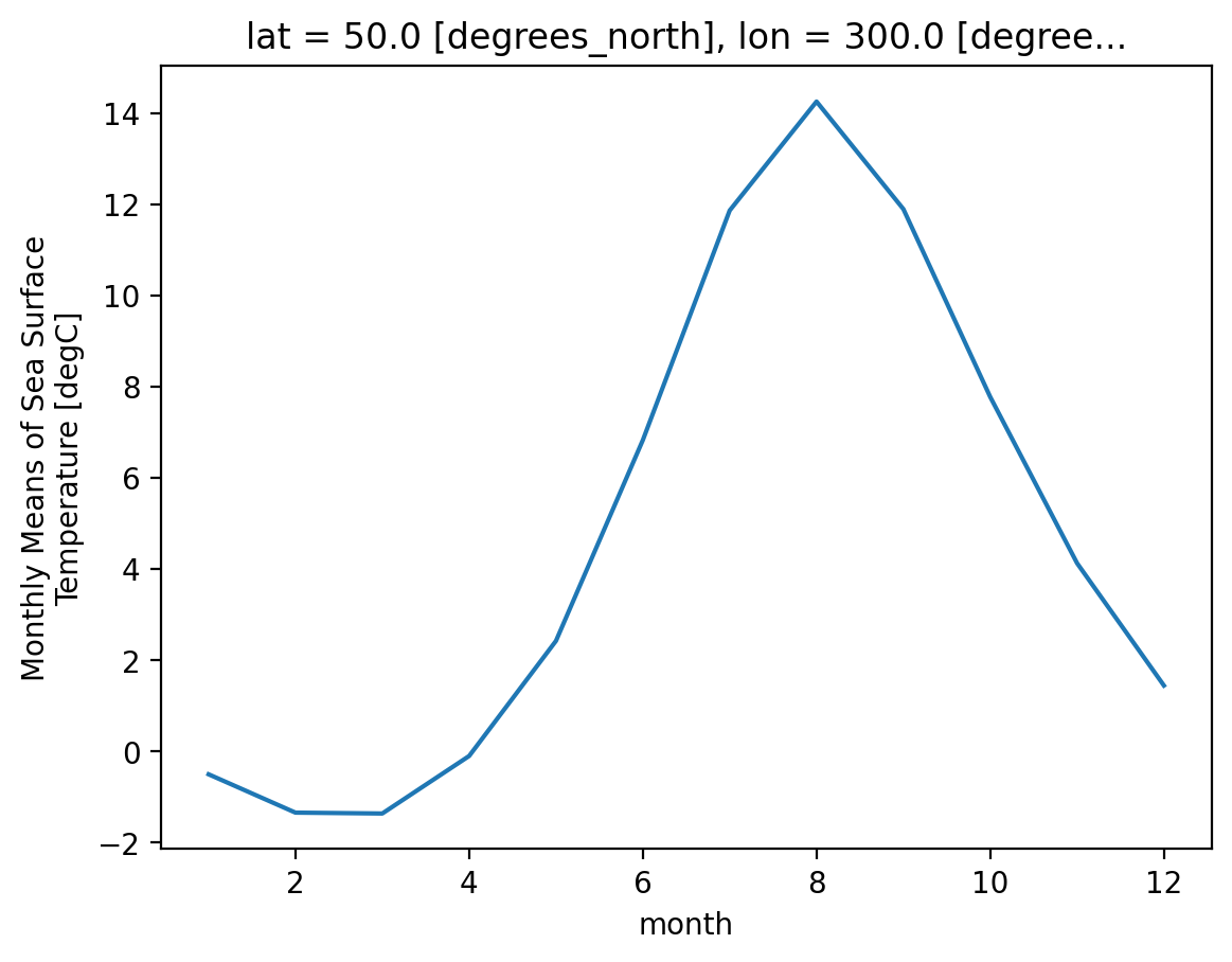
Climatology at a specific point in the North Atlantic
ds_mm.sst.sel(lon=300, lat=50).plot();
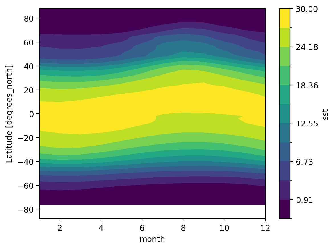
Zonal Mean Climatology
ds_mm.sst.mean(dim="lon").plot.contourf(x="month", levels=12, vmin=-2, vmax=30);
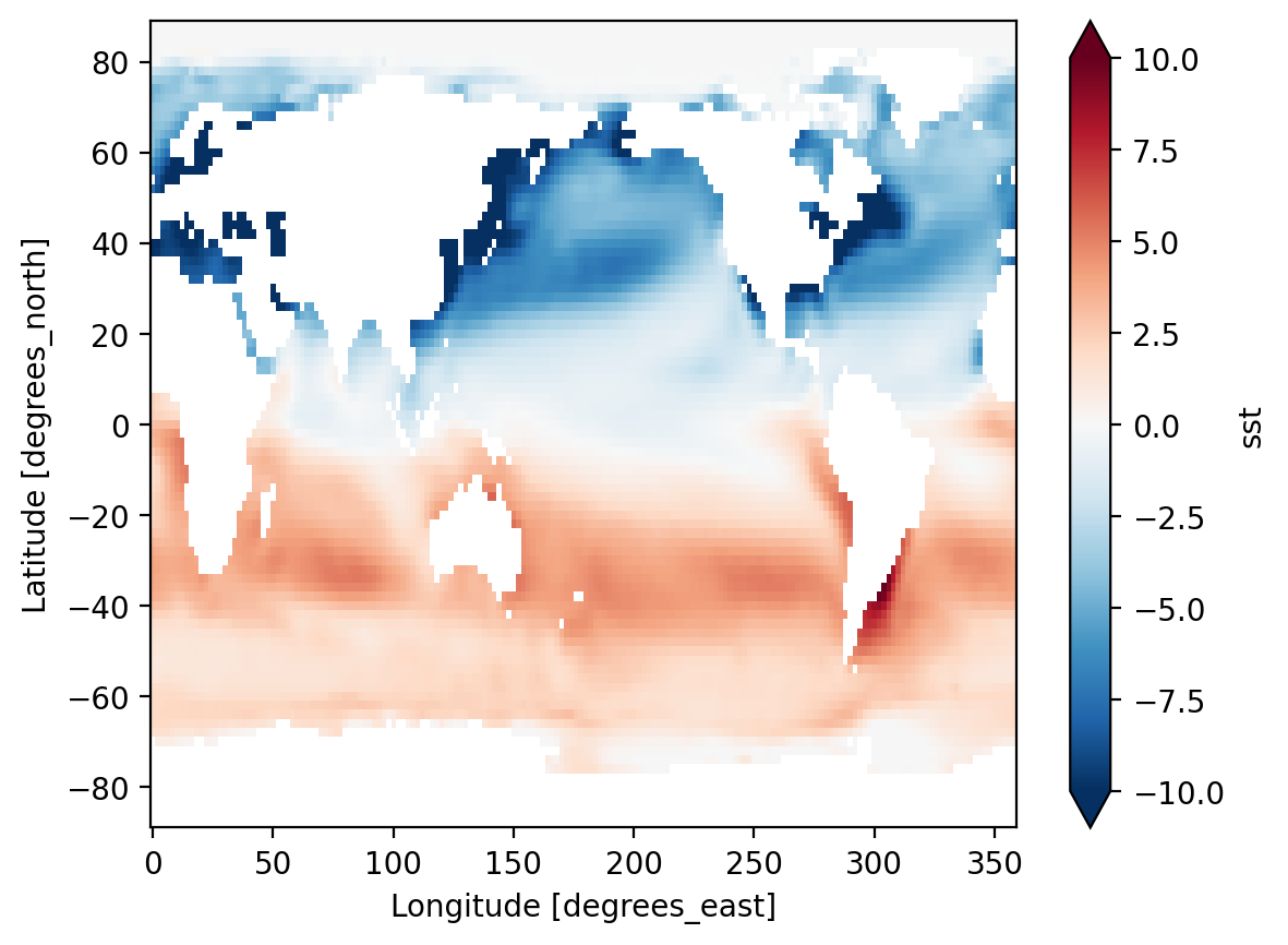
Difference between January and July Climatology
(ds_mm.sst.sel(month=1) - ds_mm.sst.sel(month=7)).plot(vmax=10);
Custom Aggregations#
The most fundamental way to apply a function and combine the results together to use the .map method.
?gb.map
.map accepts as its argument a function that expects and returns xarray
objects. We define a custom function. This function takes a single argument–the
group dataset–and returns a new dataset to be combined:
def time_mean(a):
    return a.mean(dim="time")


gb.map(time_mean)
<xarray.Dataset> Size: 770kB
Dimensions:    (month: 12, nbnds: 2, lat: 89, lon: 180)
Coordinates:
  * lat        (lat) float32 356B 88.0 86.0 84.0 82.0 ... -84.0 -86.0 -88.0
  * lon        (lon) float32 720B 0.0 2.0 4.0 6.0 ... 352.0 354.0 356.0 358.0
  * month      (month) int64 96B 1 2 3 4 5 6 7 8 9 10 11 12
Dimensions without coordinates: nbnds
Data variables:
    time_bnds  (month, nbnds) float64 192B 9.969e+36 9.969e+36 ... 9.969e+36
sst (month, lat, lon) float32 769kB -1.8 -1.8 -1.8 ... nan nan nanThis is identical to gb.mean()
Apply by iteration#
We can manually iterate over the group. The iterator returns the key (group name) and the value (the actual dataset corresponding to that group) for each group.
You could apply any function you want in the loop but you would have to manually combine the results together.
for group_name, group_ds in gb:
    # stop iterating after the first loop
    break
print(group_name)
group_ds
1
<xarray.Dataset> Size: 3MB
Dimensions:    (lat: 89, lon: 180, time: 52, nbnds: 2)
Coordinates:
  * lat        (lat) float32 356B 88.0 86.0 84.0 82.0 ... -84.0 -86.0 -88.0
  * lon        (lon) float32 720B 0.0 2.0 4.0 6.0 ... 352.0 354.0 356.0 358.0
  * time       (time) datetime64[ns] 416B 1970-01-01 1971-01-01 ... 2021-01-01
Dimensions without coordinates: nbnds
Data variables:
    time_bnds  (time, nbnds) float64 832B 9.969e+36 9.969e+36 ... 9.969e+36
    sst        (time, lat, lon) float32 3MB -1.8 -1.8 -1.8 -1.8 ... nan nan nan
Attributes: (37)Transformations#
Now we want to remove this climatology from the dataset, to examine the residual, called the anomaly, which is the interesting part from a climate perspective. Removing the seasonal climatology is a perfect example of a transformation: it operates over a group, but doesn’t change the size of the dataset. Here is one way to code it
def remove_time_mean(x):
    return x - x.mean(dim="time")


ds_anom = ds.groupby("time.month").map(remove_time_mean)
ds_anom
<xarray.Dataset> Size: 40MB
Dimensions:    (time: 624, nbnds: 2, lat: 89, lon: 180)
Coordinates:
  * lat        (lat) float32 356B 88.0 86.0 84.0 82.0 ... -84.0 -86.0 -88.0
  * lon        (lon) float32 720B 0.0 2.0 4.0 6.0 ... 352.0 354.0 356.0 358.0
  * time       (time) datetime64[ns] 5kB 1970-01-01 1970-02-01 ... 2021-12-01
Dimensions without coordinates: nbnds
Data variables:
    time_bnds  (time, nbnds) float64 10kB 0.0 0.0 0.0 0.0 ... 0.0 0.0 0.0 0.0
sst (time, lat, lon) float32 40MB 0.0 0.0 0.0 0.0 ... nan nan nan nanXarray makes these sorts of transformations easy by supporting groupby arithmetic. This concept is easiest explained with an example:
gb = ds.groupby("time.month")
ds_anom = gb - gb.mean()
ds_anom
<xarray.Dataset> Size: 40MB
Dimensions:    (lat: 89, lon: 180, time: 624, nbnds: 2)
Coordinates:
  * lat        (lat) float32 356B 88.0 86.0 84.0 82.0 ... -84.0 -86.0 -88.0
  * lon        (lon) float32 720B 0.0 2.0 4.0 6.0 ... 352.0 354.0 356.0 358.0
  * time       (time) datetime64[ns] 5kB 1970-01-01 1970-02-01 ... 2021-12-01
    month      (time) int64 5kB 1 2 3 4 5 6 7 8 9 10 ... 3 4 5 6 7 8 9 10 11 12
Dimensions without coordinates: nbnds
Data variables:
    time_bnds  (time, nbnds) float64 10kB 0.0 0.0 0.0 0.0 ... 0.0 0.0 0.0 0.0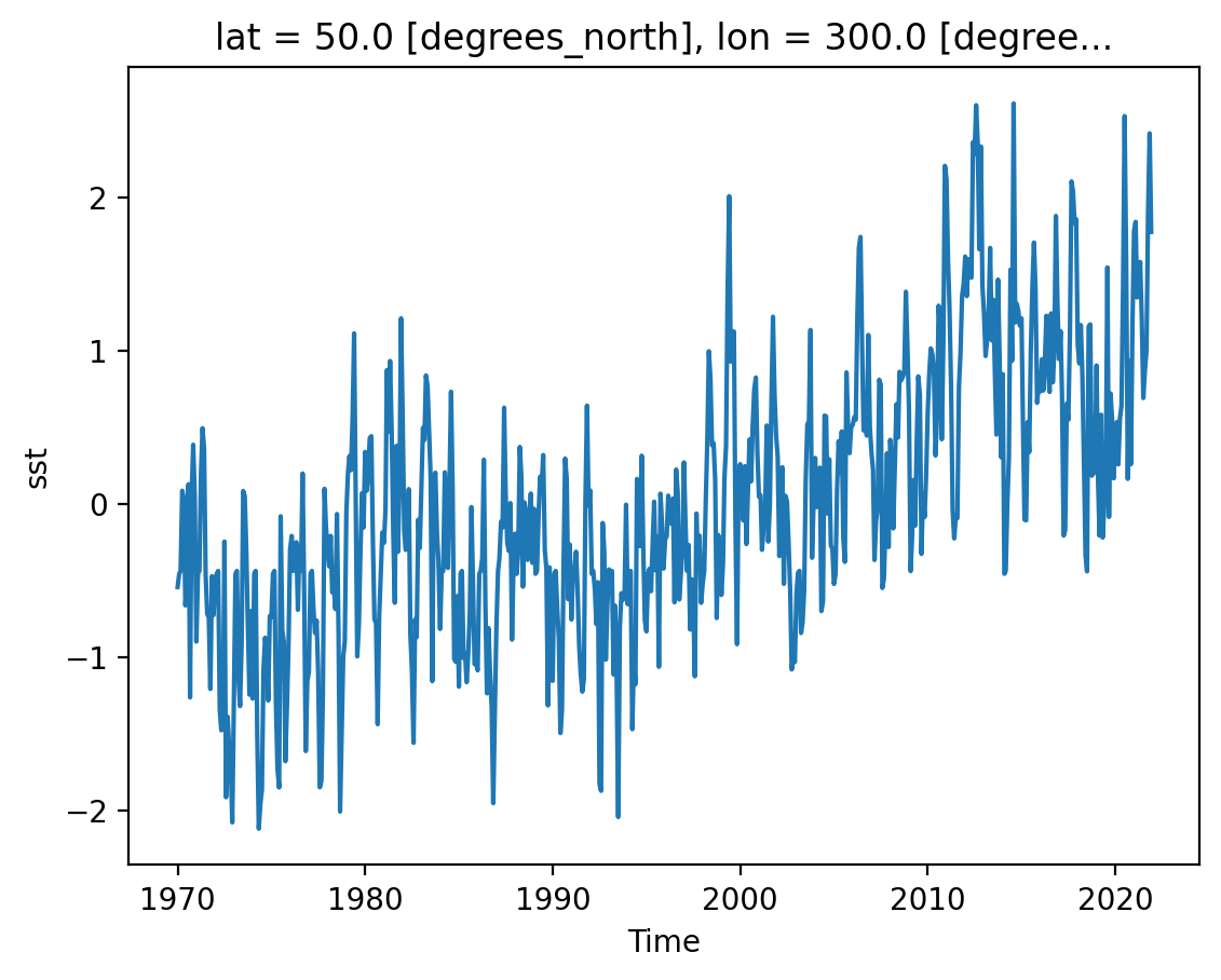
sst (time, lat, lon) float32 40MB 5.96e-07 5.96e-07 ... nan nanNow we can view the climate signal without the overwhelming influence of the seasonal cycle.
Timeseries at a single point in the North Atlantic
ds_anom.sst.sel(lon=300, lat=50).plot();
Difference between Jan. 1 2018 and Jan. 1 1970
(ds_anom.sel(time="2018-01-01") - ds_anom.sel(time="1970-01-01")).sst.plot();

Exercise
Using groupby, plot the annual mean time series of SST at 300°E, 50°N
Solution
ds.groupby("time.year").mean().sst.sel(lon=300, lat=50).plot();
Resample#
Resampling means changing the time frequency of data, usually reducing to a coarser frequency: e.g. converting daily frequency data to monthly frequency data using mean to reduce the values. This operation can be thought of as a groupby operation where each group is a single month of data. Resampling can be applied only to time-index dimensions.
First note that ds_anom has data at monthly frequency (i.e. one point every month).
ds_anom.time
<xarray.DataArray 'time' (time: 624)> Size: 5kB
1970-01-01 1970-02-01 1970-03-01 1970-04-01 ... 2021-10-01 2021-11-01 2021-12-01
Coordinates:
  * time     (time) datetime64[ns] 5kB 1970-01-01 1970-02-01 ... 2021-12-01
    month    (time) int64 5kB 1 2 3 4 5 6 7 8 9 10 11 ... 3 4 5 6 7 8 9 10 11 12
Attributes: (7)Here we compute the five-year mean along the time dimension by passing time='5Y'. '5Y' is a special frequency string. Xarray uses pandas to convert such a frequency string to a groupby operation. See the pandas documentation for how to specify a different frequency.
resample_obj = ds_anom.resample(time="5YE")
resample_obj
<DatasetResample, grouped over 1 grouper(s), 12 groups in total:
    '__resample_dim__': TimeResampler('__resample_dim__'), 12/12 groups with labels 1970-12-31, ..., 2025-12-31>
Note
resample only works with proper datetime64 coordinate labels. Note the dtype of time in the repr above.
Resampling objects are exactly like groupby objects and allow reductions, iteration, etc.
ds_anom_resample = resample_obj.mean()
ds_anom_resample
<xarray.Dataset> Size: 770kB
Dimensions:    (time: 12, nbnds: 2, lat: 89, lon: 180)
Coordinates:
  * lat        (lat) float32 356B 88.0 86.0 84.0 82.0 ... -84.0 -86.0 -88.0
  * lon        (lon) float32 720B 0.0 2.0 4.0 6.0 ... 352.0 354.0 356.0 358.0
  * time       (time) datetime64[ns] 96B 1970-12-31 1975-12-31 ... 2025-12-31
Dimensions without coordinates: nbnds
Data variables:
    time_bnds  (time, nbnds) float64 192B 0.0 0.0 0.0 0.0 ... 0.0 0.0 0.0 0.0
sst (time, lat, lon) float32 769kB -0.0005956 -0.0005648 ... nan nanfor label, group in resample_obj:
break
print(label, "\n\n", group)
1970-12-31T00:00:00.000000000

 <xarray.Dataset> Size: 770kB
Dimensions:    (lat: 89, lon: 180, time: 12, nbnds: 2)
Coordinates:
  * lat        (lat) float32 356B 88.0 86.0 84.0 82.0 ... -84.0 -86.0 -88.0
  * lon        (lon) float32 720B 0.0 2.0 4.0 6.0 ... 352.0 354.0 356.0 358.0
  * time       (time) datetime64[ns] 96B 1970-01-01 1970-02-01 ... 1970-12-01
    month      (time) int64 96B 1 2 3 4 5 6 7 8 9 10 11 12
Dimensions without coordinates: nbnds
Data variables:
    time_bnds  (time, nbnds) float64 192B 0.0 0.0 0.0 0.0 ... 0.0 0.0 0.0 0.0
    sst        (time, lat, lon) float32 769kB 5.96e-07 5.96e-07 ... nan nan
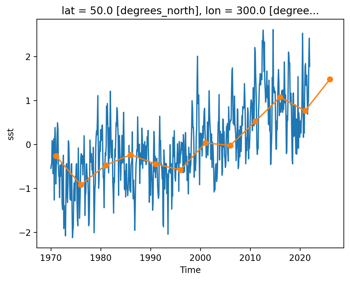
ds_anom.sst.sel(lon=300, lat=50).plot()
ds_anom_resample.sst.sel(lon=300, lat=50).plot(marker="o");
Exercise
Using resample, plot the annual mean time series of SST at 300°E, 50°N.
Compare this output to the groupby output. What differences do you see?
Solution
resampled = ds.resample(time='YE').mean().sst.sel(lon=300, lat=50)
resampled.plot();
GroupBy vs Resample#
Let’s compare the grouped and resampled outputs.
Note the different dimension names: when grouped,
timeis renamed toyear. When resampled, thetimedimension name is preservedThe values for
yearare integers, while those forresampled.timeare timestamps, similar to the input datasetBut all values are equal
from IPython.display import display_html

grouped = ds.groupby("time.year").mean().sst.sel(lon=300, lat=50)
resampled = ds.resample(time="Y").mean().sst.sel(lon=300, lat=50)
display_html(grouped)
display_html(resampled)
/home/runner/work/xarray-tutorial/xarray-tutorial/.pixi/envs/default/lib/python3.12/site-packages/xarray/groupers.py:509: FutureWarning: 'Y' is deprecated and will be removed in a future version, please use 'YE' instead.
  self.index_grouper = pd.Grouper(
<xarray.DataArray 'sst' (year: 52)> Size: 208B
4.513 4.354 3.557 4.069 3.565 3.755 4.262 ... 5.812 5.82 5.307 5.131 5.649 6.264
Coordinates:
    lat      float32 4B 50.0
    lon      float32 4B 300.0
  * year     (year) int64 416B 1970 1971 1972 1973 1974 ... 2018 2019 2020 2021
Attributes: (9)<xarray.DataArray 'sst' (time: 52)> Size: 208B
4.513 4.354 3.557 4.069 3.565 3.755 4.262 ... 5.812 5.82 5.307 5.131 5.649 6.264
Coordinates:
lat float32 4B 50.0
lon float32 4B 300.0
* time (time) datetime64[ns] 416B 1970-12-31 1971-12-31 ... 2021-12-31
Attributes: (9)np.array_equal(grouped.data, resampled.data)
True
Going further#
Follow the tutorial on high-level computation patterns