Faceting

Faceting is the art of presenting “small multiples” of the data. It is an effective way of visualizing variations of 3D data where 2D slices are visualized in a panel (subplot) and the third dimensions is varied between panels (subplots).

Here is where xarray really augments matplotlib’s functionality. We will use monthly means to illustrate

import matplotlib as mpl
import matplotlib.pyplot as plt
import numpy as np
import xarray as xr

%config InlineBackend.figure_format='retina'

ds = xr.tutorial.open_dataset("air_temperature_gradient")
monthly_means = ds.groupby("time.month").mean()
# xarray's groupby reductions drop attributes. Let's assign them back so we get nice labels.
monthly_means.Tair.attrs = ds.Tair.attrs

Note that the dimensions are now lat, lon, month.

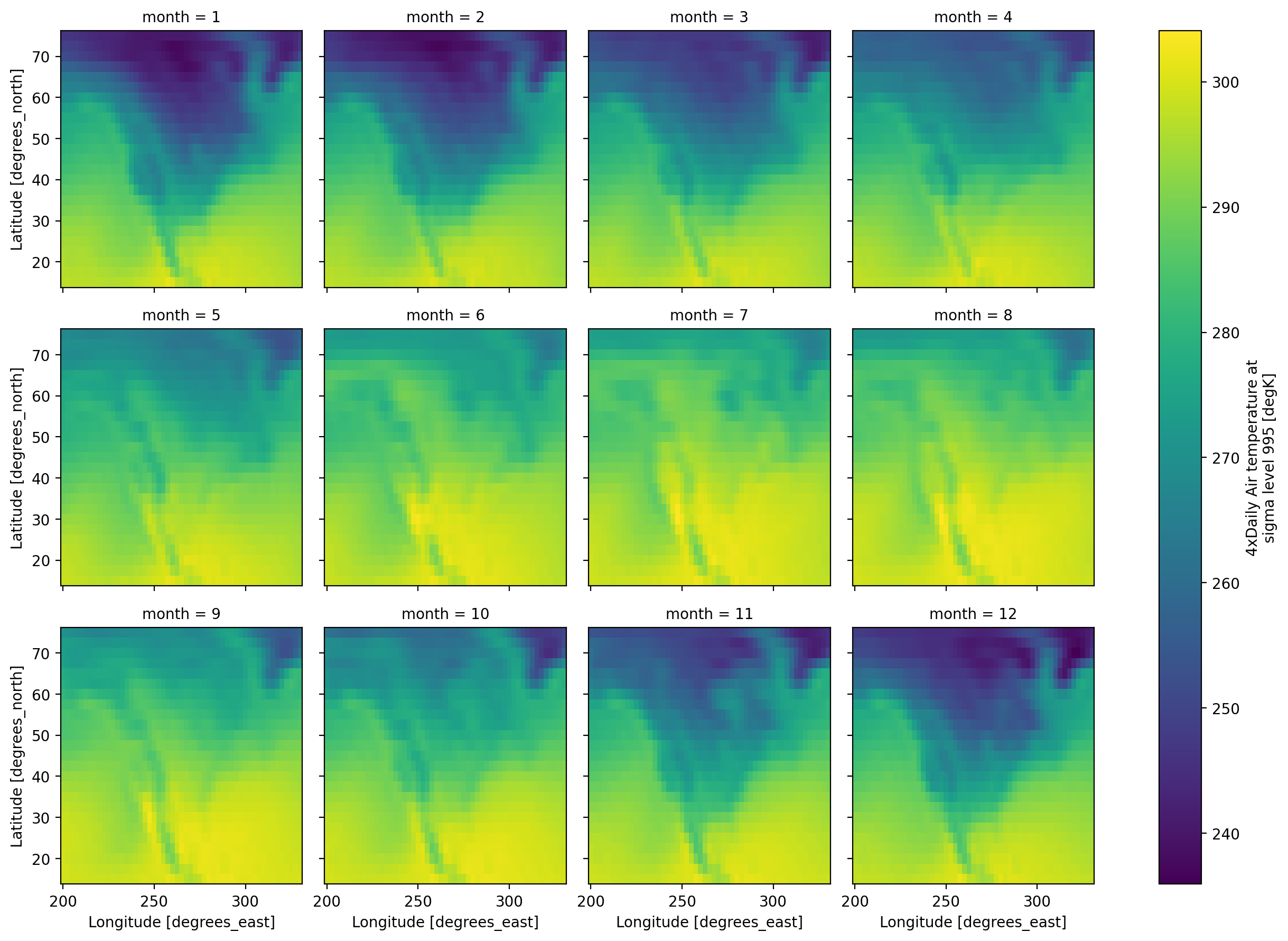
Basic faceting

We want to visualize how the monthly mean air temperature varies with month of the year.

The simplest way to facet is to specify the row or col kwargs which are expected to be a dimension name. Here we use month so that each panel or “facet” of the plot presents the mean temperature field in a given month. Since a 12 column plot would be too small to interpret, we can “wrap” the facets into multiple rows using col_wrap

fg = monthly_means.Tair.plot(
    col="month",
    col_wrap=4,  # each row has a maximum of 4 columns
)

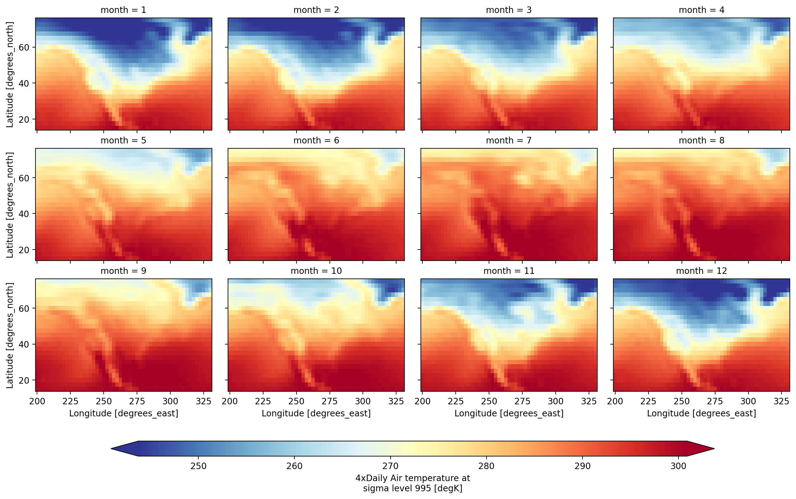
Customizing

All the usual customizations are possible

fg = monthly_means.Tair.plot(
    col="month",
    col_wrap=4,
    # The remaining kwargs customize the plot just as for not-faceted plots
    robust=True,
    cmap=mpl.cm.RdYlBu_r,
    cbar_kwargs={
        "orientation": "horizontal",
        "shrink": 0.8,
        "aspect": 40,
        "pad": 0.1,
    },
)

The returned FacetGrid object fg has many useful properties and methods e.g.

1. fg.fig provides a handle to the figure

2. fg.axes is a numpy object array with handles to each individual axes

3. fg.set_xlabels and fg.set_ylabels can be used to change axes labels.

See the documentation for a full list.

Exercise

Use these methods to set a title for the figure using suptitle, as well as change the x- and y-labels.

fg

<xarray.plot.facetgrid.FacetGrid at 0x7f63c5e56850>

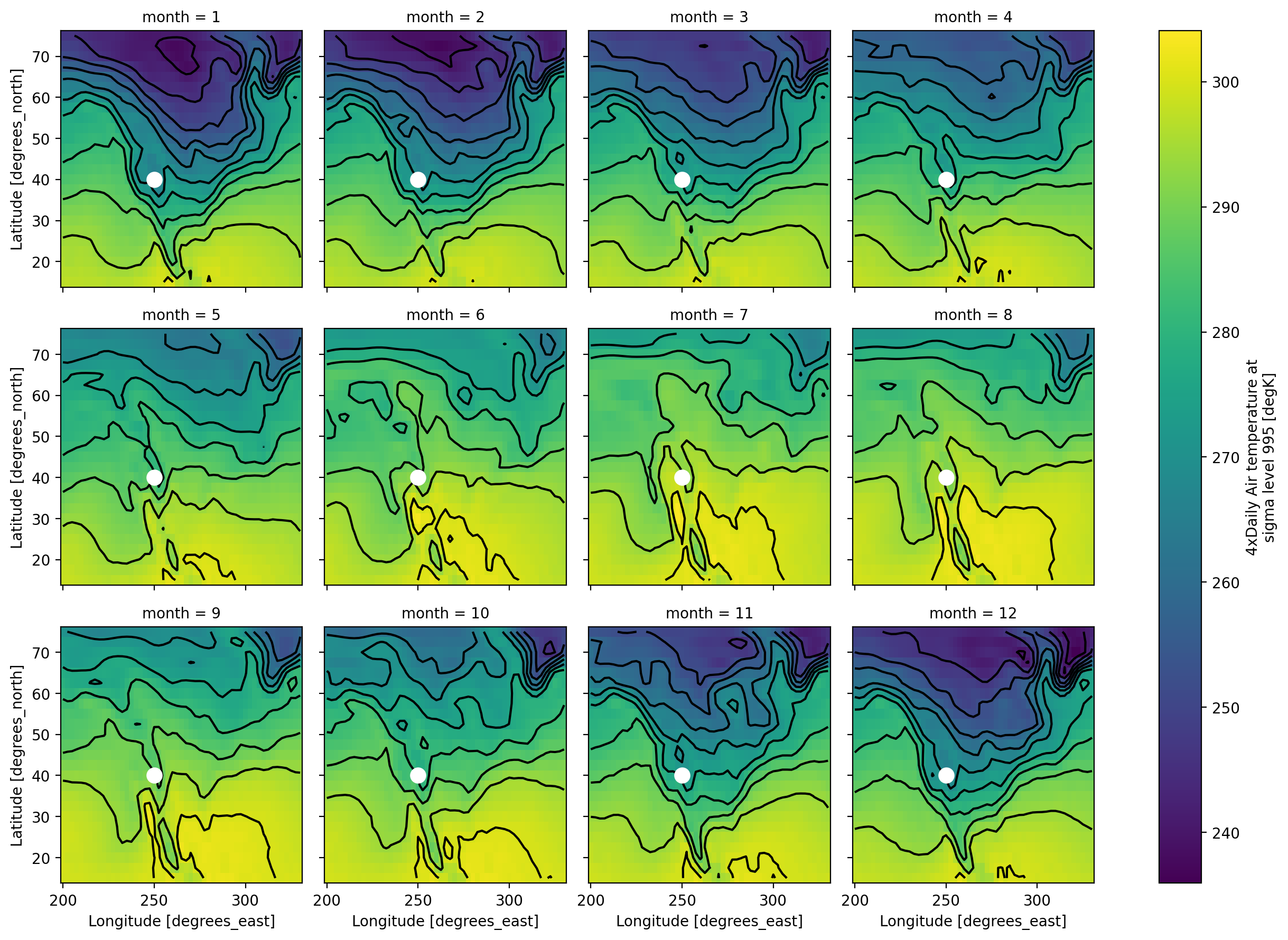
Modifying all facets

The FacetGrid object has some more advanced methods that let you customize the plot further.

Here we illustrate the use of map and map_dataarray that let you map custom plotting functions to an existing FacetGrid. The functions passed to map and map_dataarray must have a particular signature. See the docstring for more details.

Alternatively one can loop over fg.axes and modify each individual subplot as needed

fg = monthly_means.Tair.plot(col="month", col_wrap=4)

# Use this to plot contours on each panel
# Note that this plotting call uses the original DataArray gradients
fg.map_dataarray(xr.plot.contour, x="lon", y="lat", colors="k", levels=13, add_colorbar=False)

# Add a point (or anything else!)
fg.map(lambda: plt.plot(250, 40, markersize=20, marker=".", color="w"))

<xarray.plot.facetgrid.FacetGrid at 0x7f63c1ab7a10>

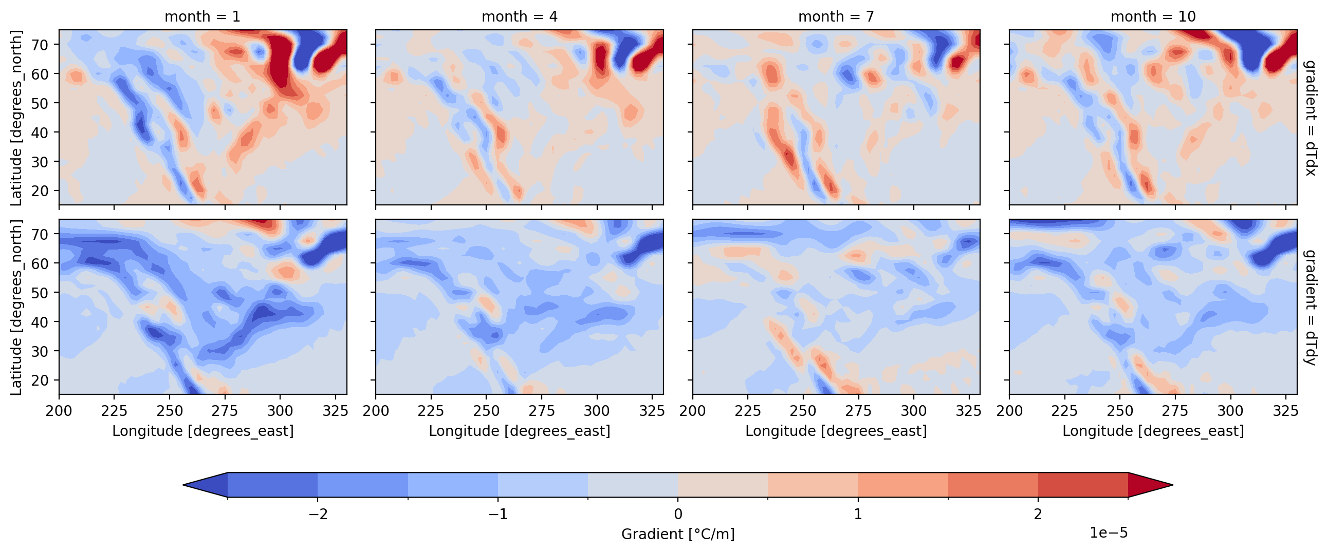
Faceting multiple DataArrays

Faceting can be used to plot multiple DataArrays in a Dataset. The trick is to use to_array() to convert a Dataset to a DataArray and then facet that.

This trick only works when it is sensible to use the same colormap and color scale for all DataArrays like with dTdx and dTdy

gradients = monthly_means[["dTdx", "dTdy"]].to_array("gradient")
gradients

<xarray.DataArray (gradient: 2, month: 12, lat: 25, lon: 53)>
array([[[[ 5.08173684e-07, -9.46942578e-07, -4.03479180e-06, ...,
           1.00858488e-05,  1.81633768e-05,  2.19007525e-05],
         [ 6.02189118e-07, -8.90132014e-07, -4.25928238e-06, ...,
           1.44879168e-05,  3.15986872e-05,  3.92536967e-05],
         [-4.04702814e-06, -4.58570503e-06, -6.01438433e-06, ...,
           2.61500463e-05,  4.34150716e-05,  5.08334851e-05],
         ...,
         [-2.34571348e-06, -1.20601771e-06,  8.53055610e-07, ...,
          -1.45294723e-06, -2.20137940e-06, -2.35507150e-06],
         [-2.84735904e-07, -7.32893909e-07, -6.86845681e-07, ...,
          -1.83361863e-06, -1.57463614e-06, -2.10182111e-06],
         [ 3.16048641e-07, -1.98249467e-07, -4.91980586e-07, ...,
          -1.71716079e-06, -7.17862974e-07, -5.23411643e-07]],

        [[-3.81416953e-06, -5.11973212e-06, -8.09966514e-06, ...,
           1.27637104e-05,  1.81622308e-05,  2.02568535e-05],
         [-4.84793247e-07, -1.95023244e-06, -5.09623078e-06, ...,
           1.05404051e-05,  2.67223077e-05,  3.38635218e-05],
         [-5.29987710e-06, -5.99807481e-06, -7.59168552e-06, ...,
           2.05774650e-05,  3.87745931e-05,  4.66650490e-05],
...
          -1.65317442e-06, -2.42777446e-06, -1.94103222e-06],
         [-1.84547469e-06, -3.26857275e-06, -3.11111307e-06, ...,
          -1.44888838e-06, -2.25341228e-06, -3.15753573e-06],
         [-8.51903962e-07, -1.66222276e-06, -2.48365177e-06, ...,
          -2.15396517e-06, -2.12524083e-06, -3.46904199e-06]],

        [[-6.71428415e-06, -8.14977375e-06, -9.80123150e-06, ...,
           3.74177898e-06,  2.25041845e-07, -5.66836025e-06],
         [-7.73049214e-06, -6.68594612e-06, -6.57780447e-06, ...,
           3.23118388e-06, -1.69362568e-06, -8.46021612e-06],
         [-1.21043013e-05, -1.01668966e-05, -9.37458026e-06, ...,
          -2.60197321e-05, -3.02746539e-05, -3.18970924e-05],
         ...,
         [-1.97388658e-06, -2.87304010e-06, -2.76804826e-06, ...,
          -2.31021318e-06, -2.91697165e-06, -2.45591286e-06],
         [-2.12526766e-06, -3.82872440e-06, -3.59293290e-06, ...,
          -2.17964885e-06, -2.80768063e-06, -3.58095190e-06],
         [-1.57234820e-06, -2.31013792e-06, -2.78555922e-06, ...,
          -2.83686700e-06, -2.73794444e-06, -3.87158479e-06]]]],
      dtype=float32)
Coordinates:
  * lat       (lat) float32 75.0 72.5 70.0 67.5 65.0 ... 22.5 20.0 17.5 15.0
  * lon       (lon) float32 200.0 202.5 205.0 207.5 ... 322.5 325.0 327.5 330.0
  * month     (month) int64 1 2 3 4 5 6 7 8 9 10 11 12
  * gradient  (gradient) object 'dTdx' 'dTdy'
Attributes:
    Conventions:  COARDS
    title:        4x daily NMC reanalysis (1948)
    description:  Data is from NMC initialized reanalysis\n(4x/day).  These a...
    platform:     Model
    references:   http://www.esrl.noaa.gov/psd/data/gridded/data.ncep.reanaly...

xarray.DataArray

• gradient: 2
• month: 12
• lat: 25
• lon: 53

• 5.082e-07 -9.469e-07 -4.035e-06 ... -2.837e-06 -2.738e-06 -3.872e-06

  array([[[[ 5.08173684e-07, -9.46942578e-07, -4.03479180e-06, ...,
             1.00858488e-05,  1.81633768e-05,  2.19007525e-05],
           [ 6.02189118e-07, -8.90132014e-07, -4.25928238e-06, ...,
             1.44879168e-05,  3.15986872e-05,  3.92536967e-05],
           [-4.04702814e-06, -4.58570503e-06, -6.01438433e-06, ...,
             2.61500463e-05,  4.34150716e-05,  5.08334851e-05],
           ...,
           [-2.34571348e-06, -1.20601771e-06,  8.53055610e-07, ...,
            -1.45294723e-06, -2.20137940e-06, -2.35507150e-06],
           [-2.84735904e-07, -7.32893909e-07, -6.86845681e-07, ...,
            -1.83361863e-06, -1.57463614e-06, -2.10182111e-06],
           [ 3.16048641e-07, -1.98249467e-07, -4.91980586e-07, ...,
            -1.71716079e-06, -7.17862974e-07, -5.23411643e-07]],
  
          [[-3.81416953e-06, -5.11973212e-06, -8.09966514e-06, ...,
             1.27637104e-05,  1.81622308e-05,  2.02568535e-05],
           [-4.84793247e-07, -1.95023244e-06, -5.09623078e-06, ...,
             1.05404051e-05,  2.67223077e-05,  3.38635218e-05],
           [-5.29987710e-06, -5.99807481e-06, -7.59168552e-06, ...,
             2.05774650e-05,  3.87745931e-05,  4.66650490e-05],
  ...
            -1.65317442e-06, -2.42777446e-06, -1.94103222e-06],
           [-1.84547469e-06, -3.26857275e-06, -3.11111307e-06, ...,
            -1.44888838e-06, -2.25341228e-06, -3.15753573e-06],
           [-8.51903962e-07, -1.66222276e-06, -2.48365177e-06, ...,
            -2.15396517e-06, -2.12524083e-06, -3.46904199e-06]],
  
          [[-6.71428415e-06, -8.14977375e-06, -9.80123150e-06, ...,
             3.74177898e-06,  2.25041845e-07, -5.66836025e-06],
           [-7.73049214e-06, -6.68594612e-06, -6.57780447e-06, ...,
             3.23118388e-06, -1.69362568e-06, -8.46021612e-06],
           [-1.21043013e-05, -1.01668966e-05, -9.37458026e-06, ...,
            -2.60197321e-05, -3.02746539e-05, -3.18970924e-05],
           ...,
           [-1.97388658e-06, -2.87304010e-06, -2.76804826e-06, ...,
            -2.31021318e-06, -2.91697165e-06, -2.45591286e-06],
           [-2.12526766e-06, -3.82872440e-06, -3.59293290e-06, ...,
            -2.17964885e-06, -2.80768063e-06, -3.58095190e-06],
           [-1.57234820e-06, -2.31013792e-06, -2.78555922e-06, ...,
            -2.83686700e-06, -2.73794444e-06, -3.87158479e-06]]]],
        dtype=float32)

• Coordinates: (4)
  • lat
    (lat)
    float32
    75.0 72.5 70.0 ... 20.0 17.5 15.0

    standard_name :

    latitude

    long_name :

    Latitude

    units :

    degrees_north

    axis :

    Y

    array([75. , 72.5, 70. , 67.5, 65. , 62.5, 60. , 57.5, 55. , 52.5, 50. , 47.5,
           45. , 42.5, 40. , 37.5, 35. , 32.5, 30. , 27.5, 25. , 22.5, 20. , 17.5,
           15. ], dtype=float32)

  • lon
    (lon)
    float32
    200.0 202.5 205.0 ... 327.5 330.0

    standard_name :

    longitude

    long_name :

    Longitude

    units :

    degrees_east

    axis :

    X

    array([200. , 202.5, 205. , 207.5, 210. , 212.5, 215. , 217.5, 220. , 222.5,
           225. , 227.5, 230. , 232.5, 235. , 237.5, 240. , 242.5, 245. , 247.5,
           250. , 252.5, 255. , 257.5, 260. , 262.5, 265. , 267.5, 270. , 272.5,
           275. , 277.5, 280. , 282.5, 285. , 287.5, 290. , 292.5, 295. , 297.5,
           300. , 302.5, 305. , 307.5, 310. , 312.5, 315. , 317.5, 320. , 322.5,
           325. , 327.5, 330. ], dtype=float32)

  • month
    (month)
    int64
    1 2 3 4 5 6 7 8 9 10 11 12

    array([ 1,  2,  3,  4,  5,  6,  7,  8,  9, 10, 11, 12])

  • gradient
    (gradient)
    object
    'dTdx' 'dTdy'

    array(['dTdx', 'dTdy'], dtype=object)

• Indexes: (4)
  • lat
    PandasIndex

    PandasIndex(Index([75.0, 72.5, 70.0, 67.5, 65.0, 62.5, 60.0, 57.5, 55.0, 52.5, 50.0, 47.5,
           45.0, 42.5, 40.0, 37.5, 35.0, 32.5, 30.0, 27.5, 25.0, 22.5, 20.0, 17.5,
           15.0],
          dtype='float32', name='lat'))

  • lon
    PandasIndex

    PandasIndex(Index([200.0, 202.5, 205.0, 207.5, 210.0, 212.5, 215.0, 217.5, 220.0, 222.5,
           225.0, 227.5, 230.0, 232.5, 235.0, 237.5, 240.0, 242.5, 245.0, 247.5,
           250.0, 252.5, 255.0, 257.5, 260.0, 262.5, 265.0, 267.5, 270.0, 272.5,
           275.0, 277.5, 280.0, 282.5, 285.0, 287.5, 290.0, 292.5, 295.0, 297.5,
           300.0, 302.5, 305.0, 307.5, 310.0, 312.5, 315.0, 317.5, 320.0, 322.5,
           325.0, 327.5, 330.0],
          dtype='float32', name='lon'))

  • month
    PandasIndex

    PandasIndex(Index([1, 2, 3, 4, 5, 6, 7, 8, 9, 10, 11, 12], dtype='int64', name='month'))

  • gradient
    PandasIndex

    PandasIndex(Index(['dTdx', 'dTdy'], dtype='object', name='gradient'))

• Attributes: (5)

  Conventions :

  COARDS

  title :

  4x daily NMC reanalysis (1948)

  description :

  Data is from NMC initialized reanalysis (4x/day). These are the 0.9950 sigma level values.

  platform :

  Model

  references :

  http://www.esrl.noaa.gov/psd/data/gridded/data.ncep.reanalysis.html

fg = gradients.isel(month=slice(None, None, 3)).plot.contourf(
    levels=13,
    col="month",
    row="gradient",
    robust=True,
    cmap=mpl.cm.coolwarm,
    cbar_kwargs={
        "orientation": "horizontal",
        "shrink": 0.8,
        "aspect": 40,
        "label": "Gradient [°C/m]",
    },
)