Tree-Based Indexing#
See also
NDPointIndex — use KD-trees and Ball trees with xarray’s indexing system for efficient nearest-neighbor lookups on real datasets.
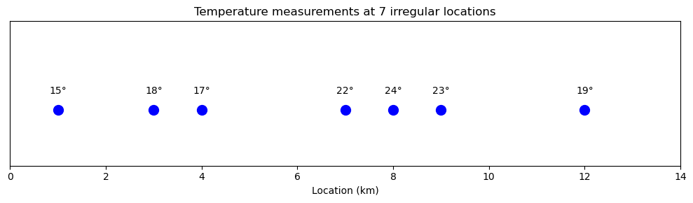
Imagine you have measurements at irregular locations and want to find the nearest data point to your query location.
In this notebook you’ll learn:
Why naive nearest-neighbor search is slow (O(n) comparisons)
How KD-trees speed this up dramatically (O(log n) comparisons)
Why KD-trees can give wrong answers for geographic lat/lon data
When to use a Ball tree instead
The nearest neighbor problem in 1D#
Let’s start with a simple 1D example:
The problem: What temperature is it at 4.7 km? We need to find the nearest measurement.
Show code cell source
Hide code cell source
import numpy as np
import matplotlib.pyplot as plt

# Temperature measurements at 7 locations along a transect
locations = np.array([1, 3, 4, 7, 8, 9, 12])
temperatures = np.array([15, 18, 17, 22, 24, 23, 19])

# Plot the data
fig, ax = plt.subplots(figsize=(10, 3))
ax.scatter(locations, np.zeros_like(locations), s=100, c='blue', zorder=5)
for loc, temp in zip(locations, temperatures):
    ax.annotate(f'{temp}°', (loc, 0.15), ha='center', fontsize=10)
ax.set_xlim(0, 14)
ax.set_ylim(-0.5, 0.8)
ax.set_xlabel('Location (km)')
ax.set_yticks([])
ax.set_title('Temperature measurements at 7 irregular locations')
plt.tight_layout()
plt.show()
The naive approach checks the distance to every point:
Show code cell source
Hide code cell source
# === Configuration: change this to explore different queries ===
query = 4.7

# Naive approach: check distance to EVERY point
fig, ax = plt.subplots(figsize=(10, 4))

# Draw the data points on the number line
ax.scatter(locations, np.zeros_like(locations), s=100, c='blue', zorder=5)
ax.scatter(query, 0, s=150, c='red', marker='x', zorder=10, lw=3)
ax.axhline(0, color='black', lw=0.5, zorder=1)

# Draw horizontal distance lines - stacked vertically for visibility
for i, loc in enumerate(locations):
    y_offset = 0.12 * (i + 1)
    # Horizontal line showing the distance
    ax.plot([query, loc], [y_offset, y_offset], 'gray', alpha=0.7, lw=2)
    # Vertical ticks at endpoints
    ax.plot([query, query], [y_offset - 0.03, y_offset + 0.03], 'gray', alpha=0.7, lw=1)
    ax.plot([loc, loc], [y_offset - 0.03, y_offset + 0.03], 'gray', alpha=0.7, lw=1)
    # Label
    ax.annotate(f'{abs(loc - query):.1f} km', ((query + loc)/2, y_offset + 0.04),
                ha='center', fontsize=8, color='gray')

ax.set_xlim(0, 14)
ax.set_ylim(-0.2, 1.1)
ax.set_xlabel('Location (km)')
ax.set_yticks([])
ax.set_title(f'Naive search: compute distance to ALL {len(locations)} points (query={query})')
plt.tight_layout()
plt.show()

print(f"Query: {query} km")
print(f"Nearest point: {locations[np.argmin(np.abs(locations - query))]} km (distance = {np.min(np.abs(locations - query)):.1f} km)")
print(f"Comparisons needed: {len(locations)}")
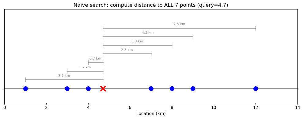
Query: 4.7 km
Nearest point: 4 km (distance = 0.7 km)
Comparisons needed: 7
With 7 points this is fine, but with millions of points this becomes slow.
The solution: Pre-compute a tree structure that partitions the space. In 1D, this is essentially a binary search tree - each split divides the remaining points in half:
Show code cell source
Hide code cell source
from scipy.spatial import KDTree
from matplotlib.patches import Rectangle

# === Configuration ===

# Build the tree (this is the pre-computation step)
tree = KDTree(locations.reshape(-1, 1))

# Query the tree first to get the result
dist, idx = tree.query([[query]])
nearest = locations[idx[0]]

# Map from value to node name for finding the result node
value_to_node = {1: 'LL', 3: 'L1', 4: 'LR', 7: 'root', 8: 'RL', 9: 'R1', 12: 'RR'}
found_node = value_to_node[nearest]

# Determine the search path based on query value
if query < 7:
    if query < 3:
        path_nodes = ['root', 'L1', 'LL']
        regions = [(0, 14), (0, 7), (0, 3)]
    else:
        path_nodes = ['root', 'L1', 'LR']
        regions = [(0, 14), (0, 7), (3, 7)]
else:
    if query < 9:
        path_nodes = ['root', 'R1', 'RL']
        regions = [(0, 14), (7, 14), (7, 9)]
    else:
        path_nodes = ['root', 'R1', 'RR']
        regions = [(0, 14), (7, 14), (9, 14)]

# Create visualization: tree on left, 3 narrowing steps on right
fig = plt.figure(figsize=(16, 9))

# Left side: Tree diagram with spatial ranges
ax_tree = fig.add_subplot(1, 2, 1)
ax_tree.set_xlim(0, 16)
ax_tree.set_ylim(-0.5, 5.5)
ax_tree.axis('off')
ax_tree.set_title('KD-tree structure\n(each node shows the spatial range it covers)', fontsize=12, fontweight='bold')

# Tree node positions - now includes spatial range for each node
nodes = {
    'root': {'pos': (8, 4.5), 'value': 7, 'color': 'steelblue', 'label': 'split=7', 'range': '[0, 14]'},
    'L1': {'pos': (4, 2.6), 'value': 3, 'color': 'coral', 'label': 'split=3', 'range': '[0, 7)'},
    'R1': {'pos': (12, 2.6), 'value': 9, 'color': 'seagreen', 'label': 'split=9', 'range': '[7, 14]'},
    'LL': {'pos': (2, 0.8), 'value': 1, 'color': 'gray', 'label': '1', 'range': '[0, 3)'},
    'LR': {'pos': (6, 0.8), 'value': 4, 'color': 'gray', 'label': '4', 'range': '[3, 7)'},
    'RL': {'pos': (10, 0.8), 'value': 8, 'color': 'gray', 'label': '8', 'range': '[7, 9)'},
    'RR': {'pos': (14, 0.8), 'value': 12, 'color': 'gray', 'label': '12', 'range': '[9, 14]'},
}

# Draw edges
edges = [('root', 'L1'), ('root', 'R1'), ('L1', 'LL'), ('L1', 'LR'), ('R1', 'RL'), ('R1', 'RR')]
for parent, child in edges:
    px, py = nodes[parent]['pos']
    cx, cy = nodes[child]['pos']
    ax_tree.plot([px, cx], [py, cy], 'k-', lw=2, zorder=1)

# Draw nodes with spatial range labels
for name, node in nodes.items():
    x, y = node['pos']
    is_split = 'split' in node['label']
    size = 2200 if is_split else 1500
    ax_tree.scatter(x, y, s=size, c=node['color'], zorder=5, edgecolors='black', linewidths=2)
    ax_tree.annotate(node['label'], (x, y), ha='center', va='center',
                     fontsize=11 if is_split else 10, fontweight='bold', color='white')
    # Add range label below each node
    ax_tree.annotate(node['range'], (x, y - 0.55), ha='center', va='top',
                     fontsize=9, color='black', style='italic',
                     bbox=dict(boxstyle='round,pad=0.2', facecolor='white', edgecolor='gray', alpha=0.8))

# Highlight the path taken
for i in range(len(path_nodes) - 1):
    px, py = nodes[path_nodes[i]]['pos']
    cx, cy = nodes[path_nodes[i+1]]['pos']
    ax_tree.plot([px, cx], [py, cy], 'r-', lw=5, alpha=0.4, zorder=2)

# Add query annotation
ax_tree.annotate(f'query={query}', (8, 4.5), xytext=(11, 5.2),
                 fontsize=11, color='red', fontweight='bold',
                 arrowprops=dict(arrowstyle='->', color='red', lw=2))

# Mark the found node
found_x, found_y = nodes[found_node]['pos']
ax_tree.annotate(f'found {nearest}!', (found_x + 1.2, found_y + 0.3), fontsize=11, ha='left', color='red', fontweight='bold')

# Right side: 3 subplots showing narrowing search space
steps = [
    ("Step 1: Start with all points", regions[0], 'steelblue', f'{query} < 7? → go left' if query < 7 else f'{query} > 7? → go right'),
    ("Step 2: After first split", regions[1], 'coral', f'{query} < 3? → go left' if query < 3 else f'{query} > 3? → go right' if query < 7 else f'{query} < 9? → go left' if query < 9 else f'{query} > 9? → go right'),
    (f"Step 3: Found nearest = {nearest}", regions[2], 'gold', None),
]

for i, (title, (region_start, region_end), color, annotation) in enumerate(steps):
    ax = fig.add_subplot(3, 2, 2*(i+1))

    # Draw all data points
    for loc in locations:
        in_region = region_start <= loc <= region_end
        ax.scatter(loc, 0, s=100 if in_region else 60,
                   c='blue' if in_region else 'lightgray',
                   zorder=5, edgecolors='black' if in_region else 'gray', linewidths=1)
        if in_region:
            ax.annotate(f'{loc}', (loc, -0.25), ha='center', fontsize=9, fontweight='bold')

    # Draw query point
    ax.scatter(query, 0, s=150, c='red', marker='x', zorder=10, lw=3)

    # Highlight the active region
    rect = Rectangle((region_start, -0.15), region_end - region_start, 0.3,
                      fill=True, facecolor=color, alpha=0.2, edgecolor=color, lw=2, zorder=2)
    ax.add_patch(rect)

    # Draw split lines
    if i == 0:
        ax.axvline(7, color='steelblue', lw=2, ls='--', alpha=0.8)
        ax.annotate('split=7', (7, 0.25), ha='center', fontsize=9, color='steelblue', fontweight='bold')
    elif i == 1:
        if query < 7:
            ax.axvline(3, color='coral', lw=2, ls='--', alpha=0.8)
            ax.annotate('split=3', (3, 0.25), ha='center', fontsize=9, color='coral', fontweight='bold')
        else:
            ax.axvline(9, color='seagreen', lw=2, ls='--', alpha=0.8)
            ax.annotate('split=9', (9, 0.25), ha='center', fontsize=9, color='seagreen', fontweight='bold')

    # Add decision annotation
    if annotation:
        ax.annotate(annotation, (0.98, 0.95), xycoords='axes fraction', ha='right', va='top',
                    fontsize=10, color='darkgreen', fontweight='bold',
                    bbox=dict(boxstyle='round', facecolor='lightyellow', edgecolor='green', alpha=0.8))

    ax.set_xlim(-0.5, 14.5)
    ax.set_ylim(-0.4, 0.45)
    ax.set_title(title, fontsize=11, fontweight='bold')
    ax.set_yticks([])
    if i == 2:
        ax.set_xlabel('Location (km)', fontsize=10)

plt.tight_layout()
plt.show()

print(f"Nearest point: {nearest} km")
print(f"Comparisons needed: ~{len(path_nodes)} (log₂({len(locations)}) ≈ 3)")
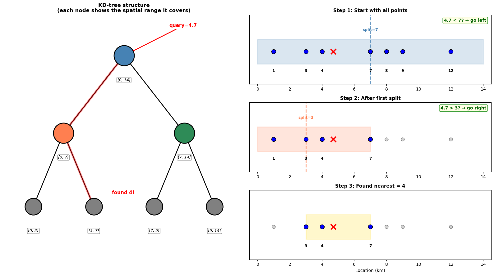
Nearest point: 4 km
Comparisons needed: ~3 (log₂(7) ≈ 3)
Extending to 2D#
The same idea works in higher dimensions. Now our measurements are scattered across a 2D area:
Show code cell source
Hide code cell source
# 2D example: temperature measurements scattered across an area
from matplotlib.patches import Rectangle

np.random.seed(42)
points_2d = np.random.rand(20, 2) * 10  # 20 points in a 10x10 area

# === Configuration ===
query_2d = np.array([6.5, 4.0])  # Change this to query a different location

# Build tree - using leafsize=2 to demonstrate meaningful subdivision
# (default leafsize=10 would barely split with only 20 points!)
LEAFSIZE = 2
tree_2d = KDTree(points_2d, leafsize=LEAFSIZE)
dist, idx = tree_2d.query([query_2d])
nearest_2d = points_2d[idx[0]]

# With leafsize=2, we get ~4 levels of splits (log2(20/2) ≈ 3-4)
# Let's show the first 2 splits conceptually, then the final leaf comparison

# Approximate the splits (KD-tree alternates x, y, x, y...)
x_split = np.median(points_2d[:, 0])  # ~4.0

# Determine which half based on query x
if query_2d[0] >= x_split:
    # Right half
    half_points = points_2d[points_2d[:, 0] >= x_split]
    x_decision = f"x={query_2d[0]} > {x_split:.1f}? → go right"
    x_region = (x_split, 0, 10, 10)  # (x_min, y_min, x_max, y_max)
else:
    # Left half
    half_points = points_2d[points_2d[:, 0] < x_split]
    x_decision = f"x={query_2d[0]} < {x_split:.1f}? → go left"
    x_region = (0, 0, x_split, 10)

y_split = np.median(half_points[:, 1])

# Determine which quadrant based on query y
if query_2d[1] >= y_split:
    # Upper region
    y_decision = f"y={query_2d[1]} > {y_split:.1f}? → go up"
    if query_2d[0] >= x_split:
        final_region = (x_split, y_split, 10, 10)  # top-right
    else:
        final_region = (0, y_split, x_split, 10)  # top-left
else:
    # Lower region
    y_decision = f"y={query_2d[1]} < {y_split:.1f}? → go down"
    if query_2d[0] >= x_split:
        final_region = (x_split, 0, 10, y_split)  # bottom-right
    else:
        final_region = (0, 0, x_split, y_split)  # bottom-left

# Define regions for visualization
regions = [
    (0, 0, 10, 10),      # Step 1: all points
    x_region,             # Step 2: half based on x
    final_region,         # Step 3: quadrant based on y
]

# Get actual points in final region (these are the leaf candidates)
x_min, y_min, x_max, y_max = final_region
final_candidates = [pt for pt in points_2d
                    if x_min <= pt[0] <= x_max and y_min <= pt[1] <= y_max]

# Create figure
fig, axes = plt.subplots(2, 2, figsize=(12, 10))
axes = axes.flatten()

step_titles = [
    "Step 1: Start with all 20 points",
    f"Step 2: Split on x ≈ {x_split:.1f}",
    f"Step 3: Split on y ≈ {y_split:.1f}",
    f"Step 4: Compare {len(final_candidates)} candidates in leaf"
]
step_colors = ['steelblue', 'coral', 'gold', 'limegreen']
decisions = [x_decision, y_decision, None, None]

for i, ax in enumerate(axes):
    x_min, y_min, x_max, y_max = regions[min(i, 2)]

    # Get points in current region
    points_in_region = [(pt, x_min <= pt[0] <= x_max and y_min <= pt[1] <= y_max) for pt in points_2d]

    # Draw all points
    for pt, in_region in points_in_region:
        ax.scatter(pt[0], pt[1], s=80 if in_region else 40,
                   c='blue' if in_region else 'lightgray',
                   edgecolors='black' if in_region else 'gray',
                   zorder=5, linewidths=1)

    # Draw query point
    ax.scatter(*query_2d, s=150, c='red', marker='x', zorder=10, lw=3)

    # Draw the active region
    rect = Rectangle((x_min, y_min), x_max - x_min, y_max - y_min,
                      fill=True, facecolor=step_colors[i], alpha=0.15,
                      edgecolor=step_colors[i], lw=2, zorder=2)
    ax.add_patch(rect)

    # Draw split lines
    if i >= 1:
        ax.axvline(x_split, color='steelblue', lw=2, ls='--', alpha=0.8)
        ax.annotate(f'x={x_split:.1f}', (x_split, 9.7), ha='center', fontsize=9,
                    color='steelblue', fontweight='bold')
    if i >= 2:
        # Only draw y split line in the relevant half
        if query_2d[0] >= x_split:
            ax.axhline(y_split, xmin=x_split/10, xmax=1, color='coral', lw=2, ls='--', alpha=0.8)
        else:
            ax.axhline(y_split, xmin=0, xmax=x_split/10, color='coral', lw=2, ls='--', alpha=0.8)
        ax.annotate(f'y={y_split:.1f}', (9.7, y_split + 0.2),
                    ha='right', va='bottom', fontsize=9, color='coral', fontweight='bold')

    # Final step: draw lines to ALL candidates
    if i == 3:
        for pt, in_region in points_in_region:
            if in_region:
                is_nearest = np.allclose(pt, nearest_2d)
                ax.plot([query_2d[0], pt[0]], [query_2d[1], pt[1]],
                        color='limegreen' if is_nearest else 'gray',
                        lw=3 if is_nearest else 1.5,
                        alpha=1.0 if is_nearest else 0.6,
                        zorder=6 if is_nearest else 4)

        ax.scatter(*nearest_2d, s=200, facecolors='none', edgecolors='limegreen', lw=3, zorder=15)
        ax.annotate('nearest!', (nearest_2d[0] + 0.3, nearest_2d[1] + 0.3),
                    ha='left', fontsize=10, color='green', fontweight='bold')

    # Add decision annotation
    if decisions[i]:
        ax.annotate(decisions[i], (0.98, 0.98), xycoords='axes fraction',
                    ha='right', va='top', fontsize=10, color='darkgreen', fontweight='bold',
                    bbox=dict(boxstyle='round', facecolor='lightyellow', edgecolor='green', alpha=0.9))

    ax.set_xlim(-0.5, 10.5)
    ax.set_ylim(-0.5, 10.5)
    ax.set_aspect('equal')
    ax.set_xlabel('x')
    ax.set_ylabel('y')
    ax.set_title(step_titles[i], fontsize=11, fontweight='bold')

plt.tight_layout()
plt.show()

print(f"Query: ({query_2d[0]}, {query_2d[1]})")
print(f"KDTree built with leafsize={LEAFSIZE}")
print(f"Started with {len(points_2d)} points")
print(f"After 2 tree splits: narrowed to {len(final_candidates)} candidates")
print(f"Final step: {len(final_candidates)} distance calculations")
print(f"Total: 2 splits + {len(final_candidates)} comparisons = {2 + len(final_candidates)} operations (vs 20 naive)")
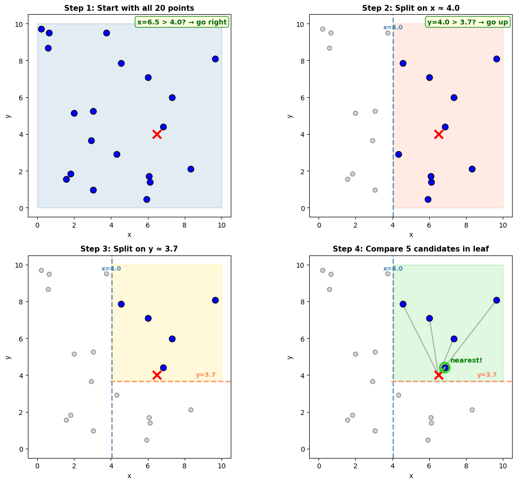
Query: (6.5, 4.0)
KDTree built with leafsize=2
Started with 20 points
After 2 tree splits: narrowed to 5 candidates
Final step: 5 distance calculations
Total: 2 splits + 5 comparisons = 7 operations (vs 20 naive)
How it scales#
The same principle extends to 3D, 4D, and beyond. Here’s how the number of comparisons scales:
Show code cell source
Hide code cell source
# How comparisons scale with data size
data_sizes = np.array([10, 100, 1000, 10000, 100000, 1000000])
naive_comparisons = data_sizes  # O(n)
kdtree_comparisons = np.log2(data_sizes).astype(int) + 1  # O(log n)

fig, ax = plt.subplots(figsize=(10, 5))

ax.plot(data_sizes, naive_comparisons, 'o-', color='gray', lw=2, markersize=8, label='Naive: O(n)')
ax.plot(data_sizes, kdtree_comparisons, 's-', color='steelblue', lw=2, markersize=8, label='KD-tree: O(log n)')

ax.set_xscale('log')
ax.set_yscale('log')
ax.set_xlabel('Number of data points')
ax.set_ylabel('Comparisons per query')
ax.set_title('Finding nearest neighbor: Naive vs KD-tree')
ax.legend(fontsize=11)
ax.grid(True, alpha=0.3)

# Annotate key points
for n, naive, kd in zip(data_sizes[::2], naive_comparisons[::2], kdtree_comparisons[::2]):
    ax.annotate(f'{naive:,}', (n, naive), textcoords="offset points", xytext=(0,10), ha='center', fontsize=9, color='gray')
    ax.annotate(f'{kd}', (n, kd), textcoords="offset points", xytext=(0,-15), ha='center', fontsize=9, color='steelblue')

plt.tight_layout()
plt.show()

print("With 1 million points: naive needs 1,000,000 comparisons, KD-tree needs ~20")
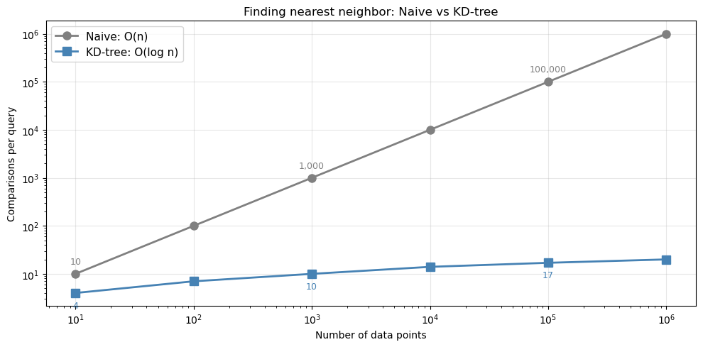
With 1 million points: naive needs 1,000,000 comparisons, KD-tree needs ~20
The problem with geographic coordinates#
KD-trees use Euclidean distance—they measure straight-line distance in whatever coordinate system you give them. This works perfectly for x/y coordinates in meters or kilometers.
But for latitude/longitude coordinates, Euclidean distance over degrees is wrong! Here’s why:
Latitude degrees are constant: 1° latitude ≈ 111 km everywhere on Earth
Longitude degrees shrink toward the poles: 1° longitude ≈ 111 km at the equator, but only ~19 km at 80°N
This means a KD-tree treating lat/lon as flat coordinates will systematically pick the wrong nearest neighbor at high latitudes:
Show code cell source
Hide code cell source
# Visualize haversine vs Euclidean - 2D circle diagram
from sklearn.neighbors import BallTree

# At 80°N (near Arctic): longitude degrees are MUCH shorter!
lat = 80
km_per_deg_lon = 111 * np.cos(np.radians(lat))  # ~19 km at 80°N!
km_per_deg_lat = 111  # always ~111 km

# Query point and two candidates (in lat/lon degrees)
query_latlon = np.array([[lat, 0]])
point_a_latlon = np.array([[lat, 2.0]])
point_b_latlon = np.array([[lat + 0.5, 0]])
points_latlon = np.vstack([point_a_latlon, point_b_latlon])

# Test both trees
kd_tree = KDTree(points_latlon)
kd_dist, kd_idx = kd_tree.query(query_latlon)
kd_picked = "A" if kd_idx[0] == 0 else "B"

ball_tree = BallTree(np.radians(points_latlon), metric='haversine')
ball_dist, ball_idx = ball_tree.query(np.radians(query_latlon))
ball_picked = "A" if ball_idx[0] == 0 else "B"

km_to_a = 2.0 * km_per_deg_lon
km_to_b = 0.5 * km_per_deg_lat

# Create figure
fig = plt.figure(figsize=(14, 10), constrained_layout=True)

# === Top: Circle diagram showing arc vs chord ===
ax_circle = fig.add_subplot(211)
ax_circle.set_aspect('equal')
ax_circle.axis('off')

# Draw circle
radius = 1
theta_full = np.linspace(0, 2*np.pi, 100)
ax_circle.plot(radius * np.cos(theta_full), radius * np.sin(theta_full), 'k-', lw=2.5)

# Two points on the circle
theta_p = np.radians(120)  # Point P
theta_q = np.radians(60)   # Point Q

p_x, p_y = radius * np.cos(theta_p), radius * np.sin(theta_p)
q_x, q_y = radius * np.cos(theta_q), radius * np.sin(theta_q)

# Draw the ARC (haversine distance) - along the circle surface
arc_theta = np.linspace(theta_q, theta_p, 50)
arc_x = radius * np.cos(arc_theta)
arc_y = radius * np.sin(arc_theta)
ax_circle.plot(arc_x, arc_y, 'r-', lw=6, solid_capstyle='round', label='Arc length (haversine)', zorder=5)

# Draw the CHORD (Euclidean distance) - straight line
ax_circle.plot([p_x, q_x], [p_y, q_y], 'b--', lw=4, label='Chord length (Euclidean)', zorder=4)

# Draw points
ax_circle.scatter([p_x, q_x], [p_y, q_y], s=250, c='dodgerblue', edgecolors='black', lw=2, zorder=10)

# Labels
ax_circle.annotate('P', (p_x - 0.18, p_y + 0.08), fontsize=24, fontweight='bold')
ax_circle.annotate('Q', (q_x + 0.1, q_y + 0.08), fontsize=24, fontweight='bold')

# Distance annotations - positioned to avoid overlap
# Arc annotation (above the arc)
arc_mid_theta = (theta_p + theta_q) / 2
arc_mid_x = 1.22 * np.cos(arc_mid_theta)
arc_mid_y = 1.22 * np.sin(arc_mid_theta)
ax_circle.annotate('arc length\n(along surface)', (arc_mid_x, arc_mid_y + 0.05),
                   fontsize=13, color='darkred', fontweight='bold', ha='center',
                   bbox=dict(boxstyle='round,pad=0.3', facecolor='mistyrose', edgecolor='red', alpha=0.9))

# Chord annotation (below the chord)
chord_mid_x = (p_x + q_x) / 2
chord_mid_y = (p_y + q_y) / 2
ax_circle.annotate('chord\n(straight line)', (chord_mid_x, chord_mid_y - 0.25),
                   fontsize=13, color='darkblue', fontweight='bold', ha='center',
                   bbox=dict(boxstyle='round,pad=0.3', facecolor='lightblue', edgecolor='blue', alpha=0.9))

# Calculate actual distances for display
arc_length = radius * abs(theta_p - theta_q)  # s = r * theta
chord_length = np.sqrt((q_x - p_x)**2 + (q_y - p_y)**2)

ax_circle.set_xlim(-1.5, 1.5)
ax_circle.set_ylim(-1.0, 1.7)
ax_circle.set_title('Haversine vs Euclidean: arc length ≠ chord length',
                    fontsize=16, fontweight='bold', pad=15)

# Legend on the left side
ax_circle.legend(loc='center left', fontsize=11, bbox_to_anchor=(-0.15, 0.3))

# Formula box on the right side
formula_text = f"Arc length > Chord length\n(arc = {arc_length:.2f},  chord = {chord_length:.2f})"
ax_circle.text(1.15, 0.3, formula_text, fontsize=12, ha='center',
               bbox=dict(boxstyle='round', facecolor='wheat', alpha=0.9))

# === Bottom row: Side-by-side comparison ===
# Bottom-left: KD-tree view (flat degrees)
ax_kd = fig.add_subplot(223)
ax_kd.scatter(0, 0, s=200, c='red', marker='x', zorder=10, lw=3, label='Query')
ax_kd.scatter(2.0, 0, s=140, c='green', zorder=5, label='Point A (2° east)')
ax_kd.scatter(0, 0.5, s=140, c='orange', zorder=5, label='Point B (0.5° north)')
ax_kd.plot([0, 2.0], [0, 0], 'g-', lw=2.5, alpha=0.7)
ax_kd.plot([0, 0], [0, 0.5], color='orange', lw=2.5, alpha=0.7)

circle_kd = plt.Circle((0, 0.5), 0.15, fill=False, color='black', lw=3, linestyle='--', zorder=15)
ax_kd.add_patch(circle_kd)
ax_kd.annotate('KD-tree picks B\n(smaller in degrees)', (0.3, 0.75), fontsize=12, fontweight='bold')

ax_kd.set_xlabel('Longitude offset (°)', fontsize=13)
ax_kd.set_ylabel('Latitude offset (°)', fontsize=13)
ax_kd.set_title(f'KD-tree: Euclidean on degrees\n(at {lat}°N latitude)', fontsize=13, fontweight='bold')
ax_kd.legend(loc='upper right', fontsize=10)
ax_kd.set_xlim(-0.5, 2.5)
ax_kd.set_ylim(-0.5, 1.2)
ax_kd.set_aspect('equal')
ax_kd.grid(True, alpha=0.3)
ax_kd.annotate('2.0°', (1.0, -0.15), ha='center', fontsize=14, color='green', fontweight='bold')
ax_kd.annotate('0.5°', (-0.25, 0.25), ha='center', fontsize=14, color='orange', fontweight='bold', rotation=90)

# Bottom-right: Reality in kilometers
ax_real = fig.add_subplot(224)
ax_real.scatter(0, 0, s=200, c='red', marker='x', zorder=10, lw=3, label=f'Query ({lat}°N)')
ax_real.scatter(km_to_a, 0, s=140, c='green', zorder=5, label='Point A')
ax_real.scatter(0, km_to_b, s=140, c='orange', zorder=5, label='Point B')
ax_real.plot([0, km_to_a], [0, 0], 'g-', lw=2.5, alpha=0.7)
ax_real.plot([0, 0], [0, km_to_b], color='orange', lw=2.5, alpha=0.7)

circle_ball = plt.Circle((km_to_a, 0), 6, fill=False, color='black', lw=3, linestyle='--', zorder=15)
ax_real.add_patch(circle_ball)
ax_real.annotate('Ball tree picks A\n(smaller in km)', (5, 55), fontsize=12, fontweight='bold')

ax_real.set_xlabel('East-West distance (km)', fontsize=13)
ax_real.set_ylabel('North-South distance (km)', fontsize=13)
ax_real.set_title(f'Ball tree: haversine (true distance)\n1° longitude = only {km_per_deg_lon:.0f} km at {lat}°N!',
                  fontsize=13, fontweight='bold')
ax_real.legend(loc='upper right', fontsize=10)
ax_real.set_xlim(-10, 70)
ax_real.set_ylim(-10, 70)
ax_real.set_aspect('equal')
ax_real.grid(True, alpha=0.3)
ax_real.annotate(f'{km_to_a:.0f} km', (km_to_a/2, -6), ha='center', fontsize=14, color='green', fontweight='bold')
ax_real.annotate(f'{km_to_b:.0f} km', (-7, km_to_b/2), ha='center', fontsize=14, color='orange', fontweight='bold', rotation=90)

plt.show()

print(f"At {lat}°N: 1° longitude = {km_per_deg_lon:.0f} km, 1° latitude = {km_per_deg_lat} km")
print(f"\nPoint A: 2° east = {km_to_a:.0f} km  (along surface)")
print(f"Point B: 0.5° north = {km_to_b:.0f} km")
print(f"\nKD-tree picked: Point {kd_picked} {'✗ WRONG!' if kd_picked == 'B' else '✓'}")
print(f"Ball tree picked: Point {ball_picked} {'✓ CORRECT!' if ball_picked == 'A' else '✗'}")
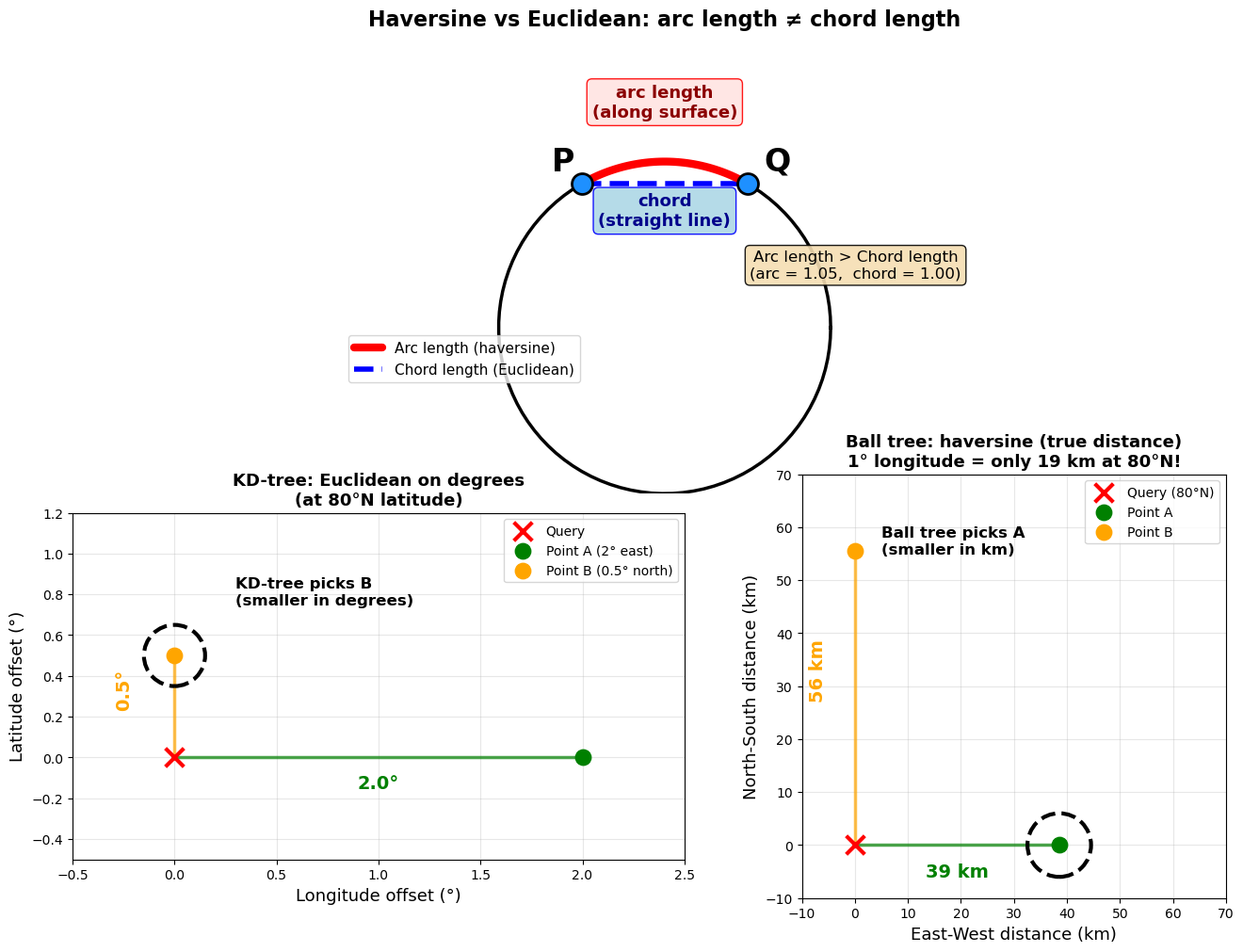
At 80°N: 1° longitude = 19 km, 1° latitude = 111 km

Point A: 2° east = 39 km  (along surface)
Point B: 0.5° north = 56 km

KD-tree picked: Point B ✗ WRONG!
Ball tree picked: Point A ✓ CORRECT!
Next steps#
Ready to use tree-based indexing with xarray? See NDPointIndex for how to integrate KD-trees and Ball trees with xarray’s indexing system.