Xarray’s Rasterio backend

In this lesson, we will learn how to use xarray’s rasterio backend engine to open GeoTIFF rasters. By the end of the lesson, we will be able to:

Learning Goals

• Learn about the GeoTIFF format

• Lean about xarray’s “rasterio” backend and the “rioxarray” accessor

• Learn how to read and plot GeoTIFF files with xarray

• Explore how to perform reprojection operations on rasters

What are GeoTIFFs?

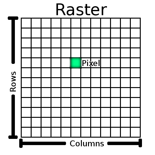
The TIFF (Tagged Image File Format) format is a metadata rich image format for raster data. GeoTIFF (Geographic Tagged Image File Format) files are TIFF files that use georeferencing information (such as map projection and coordinate systems) as metadata. A GeoTIFF file with a single band contains 2D raster data for a single characteristic (i.e., variable) and maps to a geographic region. A GeoTIFF file can have multiple bands that all map to the same geographic region.

Rasterio and Rioxarray Backends

Rasterio is a geospatial raster library that expresses GDAL (Geospatial Data Abstraction Library) data model with a Python API and CLI. Rioxarray is a wrapper around the rasterio library, that also extends the xarray api with the rio accessor. When you open a GeoTIFF file with the “rasterio” engine it returns the data as an xarray object with access to methods from the rio accessor.

Reading a GeoTIFF

Xarray’s “rasterio” backend supports reading GeoTIFFs.

Lets read a GeoTIFF file as an xr.Dataset by selecting engine='rasterio'

import xarray as xr

rds = xr.tutorial.open_dataset("RGB.byte.tif", engine="rasterio")

Note

We can also read GeoTIFFs with rioxarray.open_rasterio.

The following code snippet opens a GeoTIFF and returns a DataArray object

import rioxarray
rioxarray.open_rasterio("RGB.byte.tif")

Raster bands

GeoTIFFS can have multiple bands each representing a range or band in the electromagnetic spectrum. Arrays stored within bands in xarray are data variables and DataArray’s objects in the the Xarray Data Model.

Lets get the DataArray object (or variable) from our dataset. The variable name is “band_data”.

rda = rds["band_data"]
rda

<xarray.DataArray 'band_data' (band: 3, y: 718, x: 791)> Size: 7MB
[1703814 values with dtype=float32]
Coordinates:
  * band         (band) int64 24B 1 2 3
  * y            (y) float64 6kB 2.827e+06 2.826e+06 ... 2.612e+06 2.612e+06
  * x            (x) float64 6kB 1.021e+05 1.024e+05 ... 3.389e+05 3.392e+05
    spatial_ref  int64 8B ...
Attributes:
    AREA_OR_POINT:       Area
    STATISTICS_MAXIMUM:  255
    STATISTICS_MEAN:     29.947726688477
    STATISTICS_MINIMUM:  0
    STATISTICS_STDDEV:   52.340921626611

xarray.DataArray

'band_data'

• band: 3
• y: 718
• x: 791

• ...

  [1703814 values with dtype=float32]

• Coordinates: (4)
  • band
    (band)
    int64
    1 2 3

    array([1, 2, 3])

  • y
    (y)
    float64
    2.827e+06 2.826e+06 ... 2.612e+06

    array([2826764.979109, 2826464.937326, 2826164.895543, ..., 2612235.104457,
           2611935.062674, 2611635.020891], shape=(718,))

  • x
    (x)
    float64
    1.021e+05 1.024e+05 ... 3.392e+05

    array([102135.018963, 102435.05689 , 102735.094817, ..., 338564.905183,
           338864.94311 , 339164.981037], shape=(791,))

  • spatial_ref
    ()
    int64
    ...

    crs_wkt :

    PROJCS["WGS 84 / UTM zone 18N",GEOGCS["WGS 84",DATUM["WGS_1984",SPHEROID["WGS 84",6378137,298.257223563,AUTHORITY["EPSG","7030"]],AUTHORITY["EPSG","6326"]],PRIMEM["Greenwich",0,AUTHORITY["EPSG","8901"]],UNIT["degree",0.0174532925199433,AUTHORITY["EPSG","9122"]],AUTHORITY["EPSG","4326"]],PROJECTION["Transverse_Mercator"],PARAMETER["latitude_of_origin",0],PARAMETER["central_meridian",-75],PARAMETER["scale_factor",0.9996],PARAMETER["false_easting",500000],PARAMETER["false_northing",0],UNIT["metre",1,AUTHORITY["EPSG","9001"]],AXIS["Easting",EAST],AXIS["Northing",NORTH],AUTHORITY["EPSG","32618"]]

    semi_major_axis :

    6378137.0

    semi_minor_axis :

    6356752.314245179

    inverse_flattening :

    298.257223563

    reference_ellipsoid_name :

    WGS 84

    longitude_of_prime_meridian :

    0.0

    prime_meridian_name :

    Greenwich

    geographic_crs_name :

    WGS 84

    horizontal_datum_name :

    World Geodetic System 1984

    projected_crs_name :

    WGS 84 / UTM zone 18N

    grid_mapping_name :

    transverse_mercator

    latitude_of_projection_origin :

    0.0

    longitude_of_central_meridian :

    -75.0

    false_easting :

    500000.0

    false_northing :

    0.0

    scale_factor_at_central_meridian :

    0.9996

    spatial_ref :

    PROJCS["WGS 84 / UTM zone 18N",GEOGCS["WGS 84",DATUM["WGS_1984",SPHEROID["WGS 84",6378137,298.257223563,AUTHORITY["EPSG","7030"]],AUTHORITY["EPSG","6326"]],PRIMEM["Greenwich",0,AUTHORITY["EPSG","8901"]],UNIT["degree",0.0174532925199433,AUTHORITY["EPSG","9122"]],AUTHORITY["EPSG","4326"]],PROJECTION["Transverse_Mercator"],PARAMETER["latitude_of_origin",0],PARAMETER["central_meridian",-75],PARAMETER["scale_factor",0.9996],PARAMETER["false_easting",500000],PARAMETER["false_northing",0],UNIT["metre",1,AUTHORITY["EPSG","9001"]],AXIS["Easting",EAST],AXIS["Northing",NORTH],AUTHORITY["EPSG","32618"]]

    GeoTransform :

    101985.0 300.0379266750948 0.0 2826915.0 0.0 -300.041782729805

    [1 values with dtype=int64]

• Attributes: (5)

  AREA_OR_POINT :

  Area

  STATISTICS_MAXIMUM :

  255

  STATISTICS_MEAN :

  29.947726688477

  STATISTICS_MINIMUM :

  0

  STATISTICS_STDDEV :

  52.340921626611

Lets try getting the total number of bands for this GeoTIFF. Since rioxarray extends xarray with the rio accessor we can this accessor be able use many of the builtin rasterio methods.

rda.rio.count

3

Selection by bands

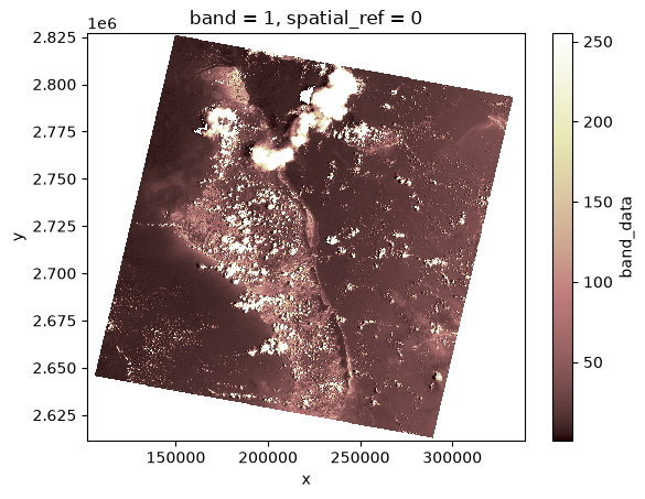
We can also select by bands. Since there are 3 bands in this dataset we can return raster array for the first band of this xr.DataArray by with indexing

Lets get the first band of this dataset and try plotting it

rda[0].plot(cmap="pink")

<matplotlib.collections.QuadMesh at 0x7f794b4af8c0>

Bounds

With .rio.bounds() we can get the spatial bounding box of our DataArray

rda.rio.bounds()

(101985.0, 2611484.9999999995, 339314.99999999994, 2826915.0)

Transformation

With .rio.transform() we can get the affine transformation matrix that maps pixel locations in (col, row) coordinates to (x, y) spatial positions.

rda.rio.transform()

Affine(300.0379266750948, 0.0, 101985.0,
       0.0, -300.041782729805, 2826915.0)

Coordinate Reference System (CRS)

We rio.crs we can get the CRS of our raster and reproject our raster.

rda.rio.crs

CRS.from_wkt('PROJCS["WGS 84 / UTM zone 18N",GEOGCS["WGS 84",DATUM["WGS_1984",SPHEROID["WGS 84",6378137,298.257223563,AUTHORITY["EPSG","7030"]],AUTHORITY["EPSG","6326"]],PRIMEM["Greenwich",0,AUTHORITY["EPSG","8901"]],UNIT["degree",0.0174532925199433,AUTHORITY["EPSG","9122"]],AUTHORITY["EPSG","4326"]],PROJECTION["Transverse_Mercator"],PARAMETER["latitude_of_origin",0],PARAMETER["central_meridian",-75],PARAMETER["scale_factor",0.9996],PARAMETER["false_easting",500000],PARAMETER["false_northing",0],UNIT["metre",1,AUTHORITY["EPSG","9001"]],AXIS["Easting",EAST],AXIS["Northing",NORTH],AUTHORITY["EPSG","32618"]]')

Reprojection

We can also reproject our raster from one CRS to another.

Lets reproject our raster from “EPSG:6326” to “EPSG:32612”

rda_reproj = rda.rio.reproject("EPSG:32612")

Note

We have to update our CRS system to the new projection with rio.write_crs. We set inplace=True to write the CRS to the existing dataset.

rda_reproj.rio.write_crs("EPSG:32612", inplace=True)

<xarray.DataArray 'band_data' (band: 3, y: 912, x: 962)> Size: 11MB
array([[[nan, nan, nan, ..., nan, nan, nan],
        [nan, nan, nan, ..., nan, nan, nan],
        [nan, nan, nan, ..., nan, nan, nan],
        ...,
        [nan, nan, nan, ..., nan, nan, nan],
        [nan, nan, nan, ..., nan, nan, nan],
        [nan, nan, nan, ..., nan, nan, nan]],

       [[nan, nan, nan, ..., nan, nan, nan],
        [nan, nan, nan, ..., nan, nan, nan],
        [nan, nan, nan, ..., nan, nan, nan],
        ...,
        [nan, nan, nan, ..., nan, nan, nan],
        [nan, nan, nan, ..., nan, nan, nan],
        [nan, nan, nan, ..., nan, nan, nan]],

       [[nan, nan, nan, ..., nan, nan, nan],
        [nan, nan, nan, ..., nan, nan, nan],
        [nan, nan, nan, ..., nan, nan, nan],
        ...,
        [nan, nan, nan, ..., nan, nan, nan],
        [nan, nan, nan, ..., nan, nan, nan],
        [nan, nan, nan, ..., nan, nan, nan]]],
      shape=(3, 912, 962), dtype=float32)
Coordinates:
  * band         (band) int64 24B 1 2 3
  * y            (y) float64 7kB 3.332e+06 3.331e+06 ... 3.017e+06 3.016e+06
  * x            (x) float64 8kB 3.828e+06 3.828e+06 ... 4.16e+06 4.16e+06
    spatial_ref  int64 8B 0
Attributes:
    AREA_OR_POINT:       Area
    STATISTICS_MAXIMUM:  255
    STATISTICS_MEAN:     29.947726688477
    STATISTICS_MINIMUM:  0
    STATISTICS_STDDEV:   52.340921626611

xarray.DataArray

'band_data'

• band: 3
• y: 912
• x: 962

• nan nan nan nan nan nan nan nan ... nan nan nan nan nan nan nan nan

  array([[[nan, nan, nan, ..., nan, nan, nan],
          [nan, nan, nan, ..., nan, nan, nan],
          [nan, nan, nan, ..., nan, nan, nan],
          ...,
          [nan, nan, nan, ..., nan, nan, nan],
          [nan, nan, nan, ..., nan, nan, nan],
          [nan, nan, nan, ..., nan, nan, nan]],
  
         [[nan, nan, nan, ..., nan, nan, nan],
          [nan, nan, nan, ..., nan, nan, nan],
          [nan, nan, nan, ..., nan, nan, nan],
          ...,
          [nan, nan, nan, ..., nan, nan, nan],
          [nan, nan, nan, ..., nan, nan, nan],
          [nan, nan, nan, ..., nan, nan, nan]],
  
         [[nan, nan, nan, ..., nan, nan, nan],
          [nan, nan, nan, ..., nan, nan, nan],
          [nan, nan, nan, ..., nan, nan, nan],
          ...,
          [nan, nan, nan, ..., nan, nan, nan],
          [nan, nan, nan, ..., nan, nan, nan],
          [nan, nan, nan, ..., nan, nan, nan]]],
        shape=(3, 912, 962), dtype=float32)

• Coordinates: (4)
  • band
    (band)
    int64
    1 2 3

    array([1, 2, 3])

  • y
    (y)
    float64
    3.332e+06 3.331e+06 ... 3.016e+06

    axis :

    Y

    long_name :

    y coordinate of projection

    standard_name :

    projection_y_coordinate

    units :

    metre

    array([3331616.539406, 3331270.443986, 3330924.348565, ..., 3017015.802088,
           3016669.706667, 3016323.611247], shape=(912,))

  • x
    (x)
    float64
    3.828e+06 3.828e+06 ... 4.16e+06

    axis :

    X

    long_name :

    x coordinate of projection

    standard_name :

    projection_x_coordinate

    units :

    metre

    array([3827578.865495, 3827924.960916, 3828271.056336, ..., 4159484.373843,
           4159830.469264, 4160176.564684], shape=(962,))

  • spatial_ref
    ()
    int64
    0

    crs_wkt :

    PROJCS["WGS 84 / UTM zone 12N",GEOGCS["WGS 84",DATUM["WGS_1984",SPHEROID["WGS 84",6378137,298.257223563,AUTHORITY["EPSG","7030"]],AUTHORITY["EPSG","6326"]],PRIMEM["Greenwich",0,AUTHORITY["EPSG","8901"]],UNIT["degree",0.0174532925199433,AUTHORITY["EPSG","9122"]],AUTHORITY["EPSG","4326"]],PROJECTION["Transverse_Mercator"],PARAMETER["latitude_of_origin",0],PARAMETER["central_meridian",-111],PARAMETER["scale_factor",0.9996],PARAMETER["false_easting",500000],PARAMETER["false_northing",0],UNIT["metre",1,AUTHORITY["EPSG","9001"]],AXIS["Easting",EAST],AXIS["Northing",NORTH],AUTHORITY["EPSG","32612"]]

    semi_major_axis :

    6378137.0

    semi_minor_axis :

    6356752.314245179

    inverse_flattening :

    298.257223563

    reference_ellipsoid_name :

    WGS 84

    longitude_of_prime_meridian :

    0.0

    prime_meridian_name :

    Greenwich

    geographic_crs_name :

    WGS 84

    horizontal_datum_name :

    World Geodetic System 1984

    projected_crs_name :

    WGS 84 / UTM zone 12N

    grid_mapping_name :

    transverse_mercator

    latitude_of_projection_origin :

    0.0

    longitude_of_central_meridian :

    -111.0

    false_easting :

    500000.0

    false_northing :

    0.0

    scale_factor_at_central_meridian :

    0.9996

    spatial_ref :

    PROJCS["WGS 84 / UTM zone 12N",GEOGCS["WGS 84",DATUM["WGS_1984",SPHEROID["WGS 84",6378137,298.257223563,AUTHORITY["EPSG","7030"]],AUTHORITY["EPSG","6326"]],PRIMEM["Greenwich",0,AUTHORITY["EPSG","8901"]],UNIT["degree",0.0174532925199433,AUTHORITY["EPSG","9122"]],AUTHORITY["EPSG","4326"]],PROJECTION["Transverse_Mercator"],PARAMETER["latitude_of_origin",0],PARAMETER["central_meridian",-111],PARAMETER["scale_factor",0.9996],PARAMETER["false_easting",500000],PARAMETER["false_northing",0],UNIT["metre",1,AUTHORITY["EPSG","9001"]],AXIS["Easting",EAST],AXIS["Northing",NORTH],AUTHORITY["EPSG","32612"]]

    GeoTransform :

    3827405.817784993 346.09542059230876 0.0 3331789.5871164217 0.0 -346.09542059230876

    array(0)

• Attributes: (5)

  AREA_OR_POINT :

  Area

  STATISTICS_MAXIMUM :

  255

  STATISTICS_MEAN :

  29.947726688477

  STATISTICS_MINIMUM :

  0

  STATISTICS_STDDEV :

  52.340921626611

Exercise

Exercise

Can you reproject and update the CRS of second band of data to ‘ESPG:3857’ and plot your results?

Solution

rda[1].rio.reproject("EPSG:3857").rio.write_crs("EPSG:3857", inplace=True).plot()