
Zarr Stores with Xarray#
Learning Objectives:#
Learn about the Zarr data format and xarray’s “zarr” backend engine
Learn how to read a Zarr store with a hierarchical structure with
xr.DataTreeLearn how to select dask arrays from a Zarr store
Explore how to use Zarr stores with xarray for computations and visualizations
What is Zarr?#
The Zarr data format is an open, community-maintained format designed for efficient, scalable storage of large N-dimensional arrays. It stores data as compressed and chunked arrays in a format well-suited to parallel processing and cloud-native workflows. Xarray’s Zarr backend allows xarray to leverage these capabilities, including the ability to store and analyze datasets far too large fit onto disk (particularly in combination with dask).
Zarr Data Organization:#
Arrays: N-dimensional arrays that can be chunked and compressed.
Groups: A container for organizing multiple arrays and other groups with a hierarchical structure.
Metadata: JSON-like metadata describing the arrays and groups, including information about data types, dimensions, chunking, compression, and user-defined key-value fields.
Dimensions and Shape: Arrays can have any number of dimensions, and their shape is defined by the number of elements in each dimension.
Coordinates & Indexing: Zarr supports coordinate arrays for each dimension, allowing for efficient indexing and slicing.
The diagram below from the Zarr v3 specification showing the structure of a Zarr store:
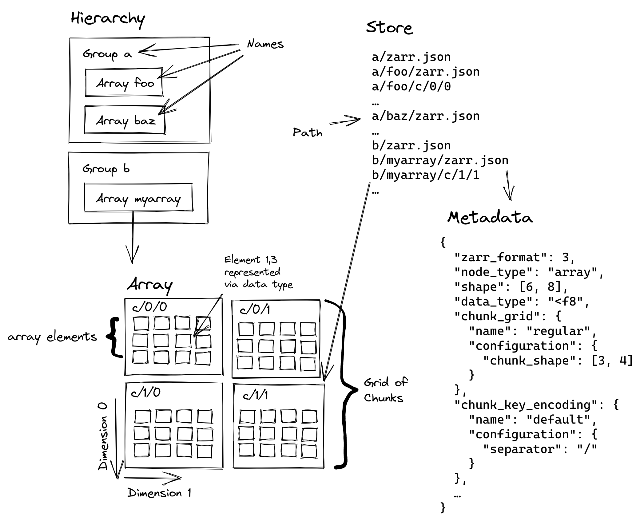
NetCDF and Zarr share similar terminology and functionality, but the key difference is that NetCDF is a single file, while Zarr is a directory-based “store” composed of many chunked files, making it better suited for distributed and cloud-based workflows.
Reading a zarr store#
With xarray’s “zarr” backend, we can read data remotely from cloud storage buckets. Since Zarr is a cloud-optimized format, our dataset is lazily-loaded as dask arrays.
The Zarr store in this tutorial is in a public storage bucket and is a precipitation dataset with a group hierarchical structure. The groups: “observed” and “reanalysis”, each contain a “precipitation” data variable derived from GPM_3IMERGHH_07 and M2T1NXFLX_5.12.4 products, respectively. The precipitation data variables in each group have different spatial resolutions that cannot be represented in a single group, so we need to read them as DataTree objects.
Let’s read in our zarr store with xr.open_datatree
import xarray as xr

precipitation_store = "https://pub-45a1d62ac8d94c4c89f4dc63681a98ed.r2.dev/precipitation.zarr"

precip_dt = xr.open_datatree(precipitation_store, engine="zarr", chunks={}, consolidated=True)
precip_dt.observed.precipitation
<xarray.DataArray 'precipitation' (time: 10, lon: 320, lat: 150)> Size: 2MB
dask.array<open_dataset-precipitation, shape=(10, 320, 150), dtype=float32, chunksize=(5, 160, 75), chunktype=numpy.ndarray>
Coordinates:
  * time     (time) datetime64[ns] 80B 2021-08-29T07:30:00 ... 2021-08-29T16:...
  * lon      (lon) float32 1kB -109.9 -109.8 -109.8 ... -78.25 -78.15 -78.05
  * lat      (lat) float32 600B 20.05 20.15 20.25 20.35 ... 34.75 34.85 34.95
Attributes:
    LongName:          \nComplete merged microwave-infrared (gauge-adjusted)\...
    Units:             mm/hr
    units:             mm/hr
    CodeMissingValue:  -9999.9
DimensionNames: time,lon,latNote
We selected "zarr" backend engine, which tells xarray to load and decode a dataset from a Zarr store. The chunks={} parameter is used to load the data into a dask array. And consolidated=True enables zarr’s consolidated metadata capability. This lets us read all of the metadata from a single file which can improve performance.
Variable selection#
With our DataTree object, we can select variables from our Zarr store with either dictionary and or attribute like syntax.
Dictionary-like interface#
precip_dt["observed/precipitation"]
<xarray.DataArray 'precipitation' (time: 10, lon: 320, lat: 150)> Size: 2MB
dask.array<open_dataset-precipitation, shape=(10, 320, 150), dtype=float32, chunksize=(5, 160, 75), chunktype=numpy.ndarray>
Coordinates:
  * time     (time) datetime64[ns] 80B 2021-08-29T07:30:00 ... 2021-08-29T16:...
  * lon      (lon) float32 1kB -109.9 -109.8 -109.8 ... -78.25 -78.15 -78.05
  * lat      (lat) float32 600B 20.05 20.15 20.25 20.35 ... 34.75 34.85 34.95
Attributes:
    LongName:          \nComplete merged microwave-infrared (gauge-adjusted)\...
    Units:             mm/hr
    units:             mm/hr
    CodeMissingValue:  -9999.9
DimensionNames: time,lon,latAttribute-like access#
precip_dt.observed.precipitation
<xarray.DataArray 'precipitation' (time: 10, lon: 320, lat: 150)> Size: 2MB
dask.array<open_dataset-precipitation, shape=(10, 320, 150), dtype=float32, chunksize=(5, 160, 75), chunktype=numpy.ndarray>
Coordinates:
  * time     (time) datetime64[ns] 80B 2021-08-29T07:30:00 ... 2021-08-29T16:...
  * lon      (lon) float32 1kB -109.9 -109.8 -109.8 ... -78.25 -78.15 -78.05
  * lat      (lat) float32 600B 20.05 20.15 20.25 20.35 ... 34.75 34.85 34.95
Attributes:
    LongName:          \nComplete merged microwave-infrared (gauge-adjusted)\...
    Units:             mm/hr
    units:             mm/hr
    CodeMissingValue:  -9999.9
DimensionNames: time,lon,latDictionary and Attribute like access#
precip_dt.observed["precipitation"]
<xarray.DataArray 'precipitation' (time: 10, lon: 320, lat: 150)> Size: 2MB
dask.array<open_dataset-precipitation, shape=(10, 320, 150), dtype=float32, chunksize=(5, 160, 75), chunktype=numpy.ndarray>
Coordinates:
  * time     (time) datetime64[ns] 80B 2021-08-29T07:30:00 ... 2021-08-29T16:...
  * lon      (lon) float32 1kB -109.9 -109.8 -109.8 ... -78.25 -78.15 -78.05
  * lat      (lat) float32 600B 20.05 20.15 20.25 20.35 ... 34.75 34.85 34.95
Attributes:
    LongName:          \nComplete merged microwave-infrared (gauge-adjusted)\...
    Units:             mm/hr
    units:             mm/hr
    CodeMissingValue:  -9999.9
DimensionNames: time,lon,latNote
All of these variable selection options return the same “precipitation” xr.DataArray object, as a chunked dask.Array, from the “observed” group of our Zarr store.
Time slicing#
We can index and subset by time on our xr.DataTree object. Each time slice in our Zarr store represents one hour of data with a total of 10 hours of data.
Let’s explore the different ways we can get the first 5 hours of data.
Label-based indexing#
Let’s try getting the first 5 hours of data with .sel(time=).
Since the time slices are ordered we can get a subset of the array of our time coordinate and pass it to the .sel method.
time_index = precip_dt.time[0:5]
precip_dt.sel(time=time_index)
<xarray.DataTree>
Group: /
│   Dimensions:  (time: 5)
│   Coordinates:
│     * time     (time) datetime64[ns] 40B 2021-08-29T07:30:00 ... 2021-08-29T11:...
├── Group: /observed
│       Dimensions:        (time: 5, lon: 320, lat: 150)
│       Coordinates:
│         * lon            (lon) float32 1kB -109.9 -109.8 -109.8 ... -78.15 -78.05
│         * lat            (lat) float32 600B 20.05 20.15 20.25 ... 34.75 34.85 34.95
│       Data variables:
│           precipitation  (time, lon, lat) float32 960kB dask.array<chunksize=(5, 160, 75), meta=np.ndarray>
└── Group: /reanalysis
        Dimensions:        (time: 5, lat: 31, lon: 52)
        Coordinates:
          * lat            (lat) float64 248B 20.0 20.5 21.0 21.5 ... 34.0 34.5 35.0
          * lon            (lon) float64 416B -110.0 -109.4 -108.8 ... -78.75 -78.12
        Data variables:
precipitation (time, lat, lon) float32 32kB dask.array<chunksize=(5, 31, 52), meta=np.ndarray>Datetime indexing#
We can also subset by time with a datetime string.
precip_dt.sel(time=slice("2021-08-29T07:30:00", "2021-08-29T16:30:00"))
<xarray.DataTree>
Group: /
│   Dimensions:  (time: 10)
│   Coordinates:
│     * time     (time) datetime64[ns] 80B 2021-08-29T07:30:00 ... 2021-08-29T16:...
├── Group: /observed
│       Dimensions:        (time: 10, lon: 320, lat: 150)
│       Coordinates:
│         * lon            (lon) float32 1kB -109.9 -109.8 -109.8 ... -78.15 -78.05
│         * lat            (lat) float32 600B 20.05 20.15 20.25 ... 34.75 34.85 34.95
│       Data variables:
│           precipitation  (time, lon, lat) float32 2MB dask.array<chunksize=(5, 160, 75), meta=np.ndarray>
└── Group: /reanalysis
        Dimensions:        (time: 10, lat: 31, lon: 52)
        Coordinates:
          * lat            (lat) float64 248B 20.0 20.5 21.0 21.5 ... 34.0 34.5 35.0
          * lon            (lon) float64 416B -110.0 -109.4 -108.8 ... -78.75 -78.12
        Data variables:
precipitation (time, lat, lon) float32 64kB dask.array<chunksize=(10, 31, 52), meta=np.ndarray>Positional Indexing#
Or by the index of our time dimension .isel(time=slice())
precip_dt.isel(time=slice(0, 5))
<xarray.DataTree>
Group: /
│   Dimensions:  (time: 5)
│   Coordinates:
│     * time     (time) datetime64[ns] 40B 2021-08-29T07:30:00 ... 2021-08-29T11:...
├── Group: /observed
│       Dimensions:        (time: 5, lon: 320, lat: 150)
│       Coordinates:
│         * lon            (lon) float32 1kB -109.9 -109.8 -109.8 ... -78.15 -78.05
│         * lat            (lat) float32 600B 20.05 20.15 20.25 ... 34.75 34.85 34.95
│       Data variables:
│           precipitation  (time, lon, lat) float32 960kB dask.array<chunksize=(5, 160, 75), meta=np.ndarray>
└── Group: /reanalysis
        Dimensions:        (time: 5, lat: 31, lon: 52)
        Coordinates:
          * lat            (lat) float64 248B 20.0 20.5 21.0 21.5 ... 34.0 34.5 35.0
          * lon            (lon) float64 416B -110.0 -109.4 -108.8 ... -78.75 -78.12
        Data variables:
precipitation (time, lat, lon) float32 32kB dask.array<chunksize=(5, 31, 52), meta=np.ndarray>Chunking#
Chunking is the process of dividing arrays into smaller pieces, which allows for parallel processing and efficient storage.
To examine the chunks in our Zarr store, with xarray you can use the chunks attribute on the xr.DataArray object.
precip_dt.observed["precipitation"].data.chunks
((5, 5), (160, 160), (75, 75))
Selecting by chunks#
Since we loaded our data as a dask.Array, we can access data from each chunked array in our Zarr store.
Let’s get the first chunk of the “observed/precipitation” variable in our zarr store.
precip_dt.observed["precipitation"].data.blocks[0, 0, 0].compute()
array([[[0.   , 0.   , 0.   , ..., 0.   , 0.   , 0.   ],
        [0.   , 0.   , 0.   , ..., 0.   , 0.   , 0.   ],
        [0.   , 0.   , 0.   , ..., 0.   , 0.   , 0.   ],
        ...,
        [0.   , 0.   , 0.   , ..., 0.   , 0.   , 0.   ],
        [0.   , 0.   , 0.   , ..., 0.   , 0.   , 0.   ],
        [0.   , 0.   , 0.   , ..., 0.   , 0.   , 0.   ]],

       [[0.   , 0.   , 0.   , ..., 0.   , 0.   , 0.   ],
        [0.   , 0.   , 0.   , ..., 0.   , 0.   , 0.   ],
        [0.   , 0.   , 0.   , ..., 0.   , 0.   , 0.   ],
        ...,
        [0.   , 0.   , 0.   , ..., 0.   , 0.   , 0.   ],
        [0.   , 0.   , 0.   , ..., 0.   , 0.   , 0.   ],
        [0.   , 0.   , 0.   , ..., 0.   , 0.   , 0.   ]],

       [[0.   , 0.   , 0.   , ..., 0.   , 0.   , 0.   ],
        [0.   , 0.   , 0.   , ..., 0.   , 0.   , 0.   ],
        [0.   , 0.   , 0.   , ..., 0.   , 0.   , 0.   ],
        ...,
        [0.   , 0.   , 0.   , ..., 0.035, 0.   , 0.   ],
        [0.   , 0.   , 0.   , ..., 0.02 , 0.005, 0.   ],
        [0.   , 0.   , 0.   , ..., 0.26 , 0.04 , 0.   ]],

       [[0.   , 0.   , 0.   , ..., 0.   , 0.   , 0.   ],
        [0.   , 0.   , 0.   , ..., 0.   , 0.   , 0.   ],
        [0.   , 0.   , 0.   , ..., 0.   , 0.   , 0.   ],
        ...,
        [0.   , 0.   , 0.   , ..., 0.   , 0.   , 0.   ],
        [0.   , 0.   , 0.   , ..., 0.   , 0.   , 0.   ],
        [0.   , 0.   , 0.   , ..., 0.   , 0.   , 0.   ]],

       [[0.   , 0.   , 0.   , ..., 0.   , 0.   , 0.   ],
        [0.   , 0.   , 0.   , ..., 0.   , 0.   , 0.   ],
        [0.   , 0.   , 0.   , ..., 0.   , 0.   , 0.   ],
        ...,
        [0.   , 0.   , 0.   , ..., 0.   , 0.   , 0.   ],
        [0.   , 0.   , 0.   , ..., 0.   , 0.   , 0.   ],
        [0.   , 0.   , 0.   , ..., 0.   , 0.   , 0.   ]]],
      shape=(5, 160, 75), dtype=float32)
Note
We added .data to our xr.DataArray to access the dask.Array. The .blocks[] method allows you to index by chunk and .compute() returns the np.ndarray.
Exercise#
Exercise
Can you calculate and plot the mean precipitation, starting at 09:55 for the reanalysis group in this zarr store?
Hint
This is how you could calculate mean “precipitation”
precip_dt.reanalysis['precipitation'].mean(dim='time')
Solution
precip_dt.reanalysis['precipitation'].sel(time=slice('2021-08-29T09:55:00', '2021-08-29T16:30:00')).mean(dim='time').plot()